TQQQ Trading Strategy (Weekly)

Today I present two TQQQ trading strategy backtest results with weekly setup with similar reward-risk but very different characteristics. TQQQ is the ProShares UltraPro QQQ, a triple leveraged ETF tracking the Nasdaq. The backtests were for the 288 weeks 2/11/10 through 8/14/15.

The first trading strategy was found by optimizing the scanner for low drawdown, (per Prasad’s request):

Backtest results for weekly TQQQ trading strategy showing low (8%) drawdown. The backtest is for the period 2/11/10 to 8/14/15.

This strategy gave similar return to buy/hold with much lower drawdown (8% vs. 41%). It only spent 42% of the time in the market, so it was quite efficient. The user defined price is found by averaging the open price of the current week, the previous week’s low price and the previous week’s high price. Here is the equity curve:

Equity curve for the low drawdown TQQQ trading strategy backtest. Return is about the same as buy/hold.

These results were corrected 1-4-2016 to fix the short-hold return.

The second TQQQ trading strategy backtest was found by optimizing the SignalSolver scanner for returns:

This is a long & short strategy when you are were always in the market either long or short. The equity curve shows that this was not a frequent trader, in fact no trades since Dec 2011:

List of trades: TQQQ.W RR .

Andrew

Please note: All trading strategies are backtested on a single security and will typically not give similar results on other securities. All returns are compounded. Trading costs are assumed to be $7.00 per trade with zero slippage.

The posting was corrected 12/29/2015 for an error in the short-side returns of the BMS ACO algorithm.

Update 10-20-2016

BMS ACO has continued to track buy-hold with no trades adding 7.45%.

TQQQ Trading Strategy Update Oct 20th 2016

TQQQ Trading Strategy Update Oct 20th 2016

This strategy peaked 11/30/2015.

OMER Trading Strategy (Daily)

Frequent reversals characterize this strategy for Omeros Corporation

This OMER trading strategy is signal rich; there were 174 dual signal days out of the 528 days in the analysis. Added to that 151 buy signal only days and 39 sell signal only days and you get 364 signal days, of which 250 were actionable signals leading to trades, of which only 146 were good. Still, all that activity led to a theoretical $311,341 profit from $10K invested over the 2 year period from 7/12/13 to 8/14/15.

The algorithm itself is a bit of an odd one with buys triggering off price changes from the open price and sells triggering off price changes from the previous day’s open price. Is it just a fluke that it has worked so consistently? In its worst quartus (132 trading days in this case) this algorithm returned 250% annualized or 93% actual return.

You can see from the list of trades and the equity chart that there were several periods of daily reversals from long to short and back again. You might think that ignoring dual signals would work better, but it doesn’t–it leads to an 80% reduction in returns.

This strategy was found by optimizing for minimum quartus returns and then doing some minor tweaking by hand, which is quite easy to do since the Scan charts in Signalsolver are interactive. I just moved the buy and sell points to areas away where there were lower returns. I’m just going to post the charts, if you need help interpreting them I would refer you to yesterday’s AAPL post where I discuss the methodology in detail.

By the way, OMER took off today gapping up 70% or so. I was working on it before that so this change doesn’t show on the data, but the proceeds would have jumped to $929,212. It would be cheating to track this strategy knowing it had already added 70%, so I’m not planning on doing so.

Andrew

OMER.D Time

Equity curve for the OMER trading strategy showing $545,057 in returns over a 2 year period.

OMER Daily Trading Strategy, sync up info

OMER Daily algorithm–current and pending trades, if you are looking for synchronization info.

Follow up 12/29/2015

This algorithm peaked and then failed dramatically immediately after the 70% gap up on Aug 18th, very shortly after publication. Here is the 528 day equity curve:

OMER.D Equity Followup

Here are the stats:


OMER.D Table Followup

Buy-hold would have been a much better option. For a profit, one solution was a buy point of 2.0% and a sell point of 4.4%, which would have given a return of $13,964 over the 94 days. Unfortunately, these parameter changes don’t appear to be predictable.

Andrew

AAPL Trading Strategy (2)

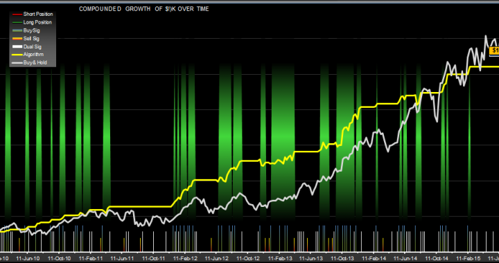
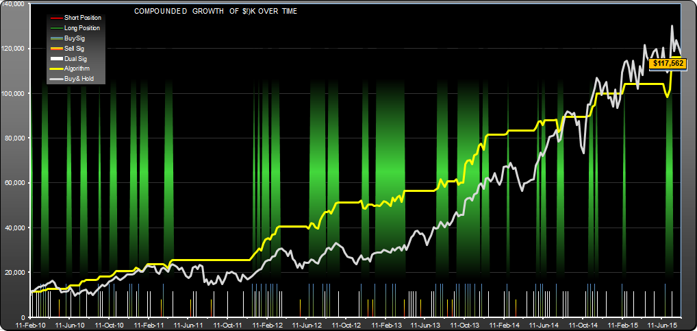
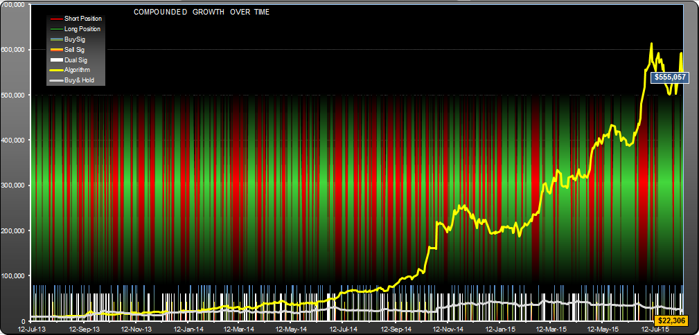
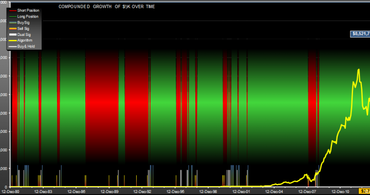
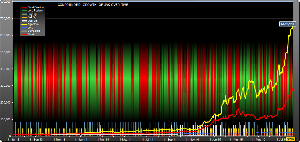
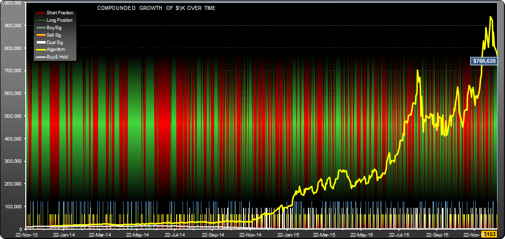
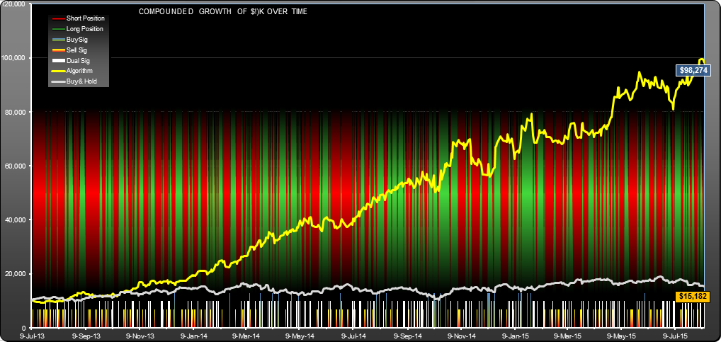
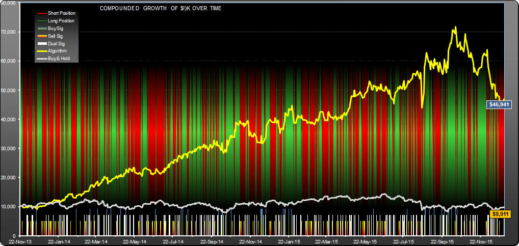
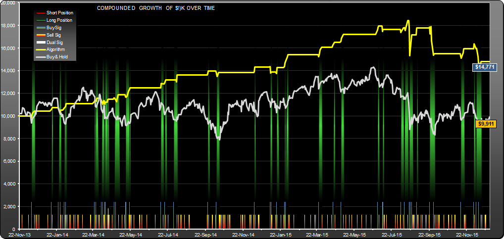
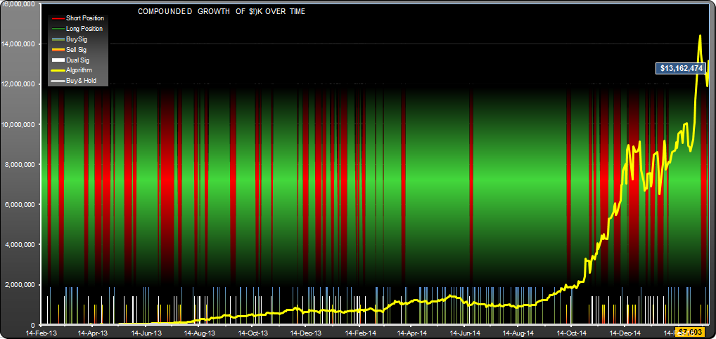
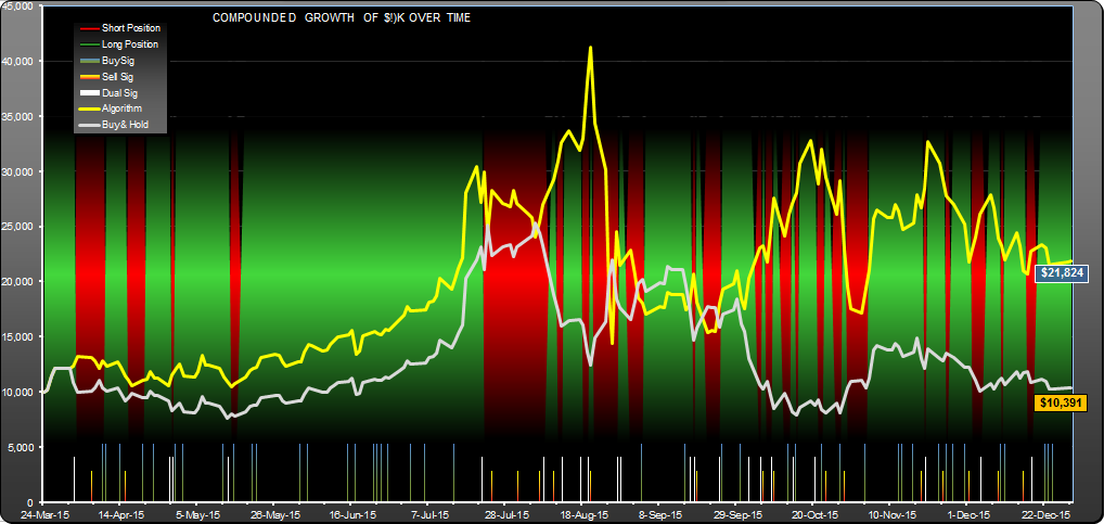
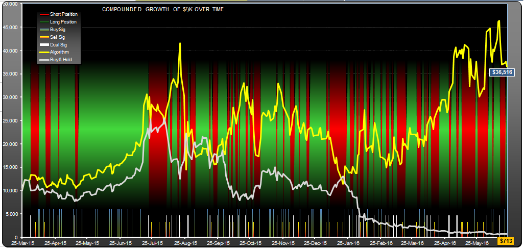
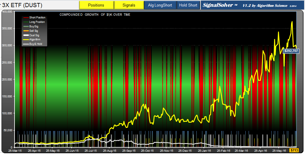
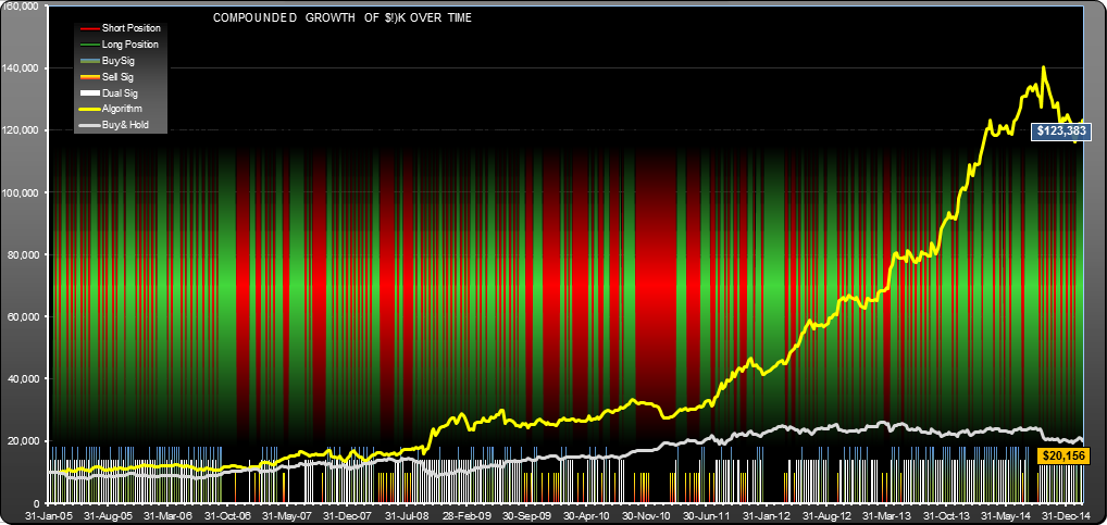
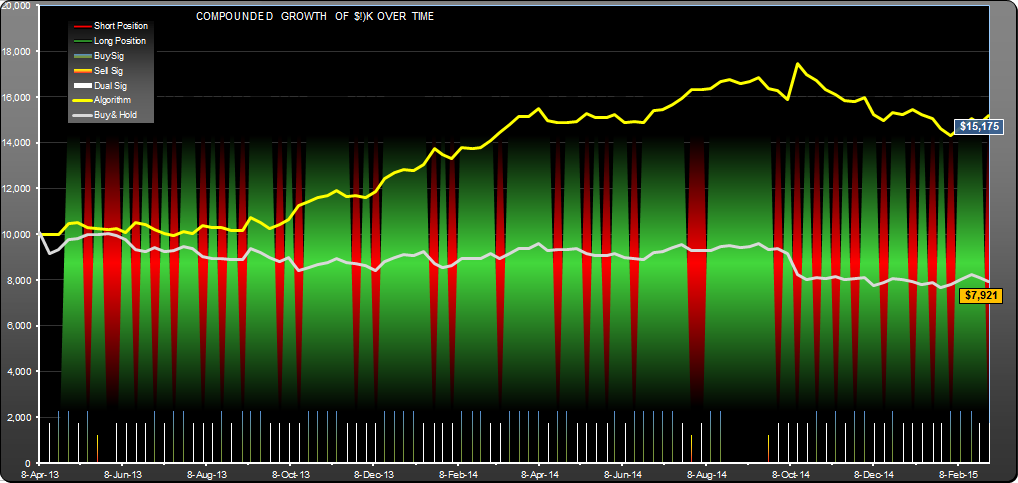
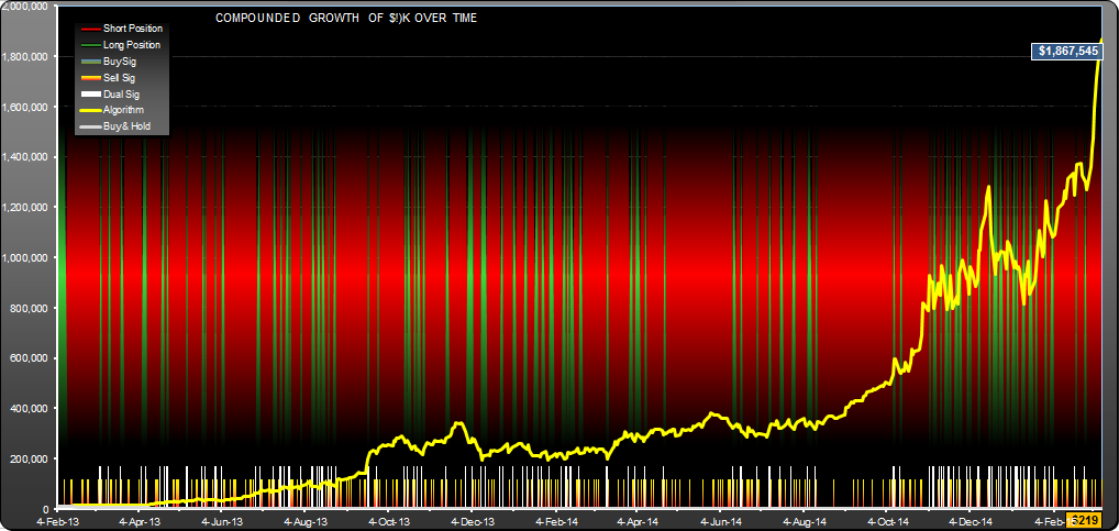
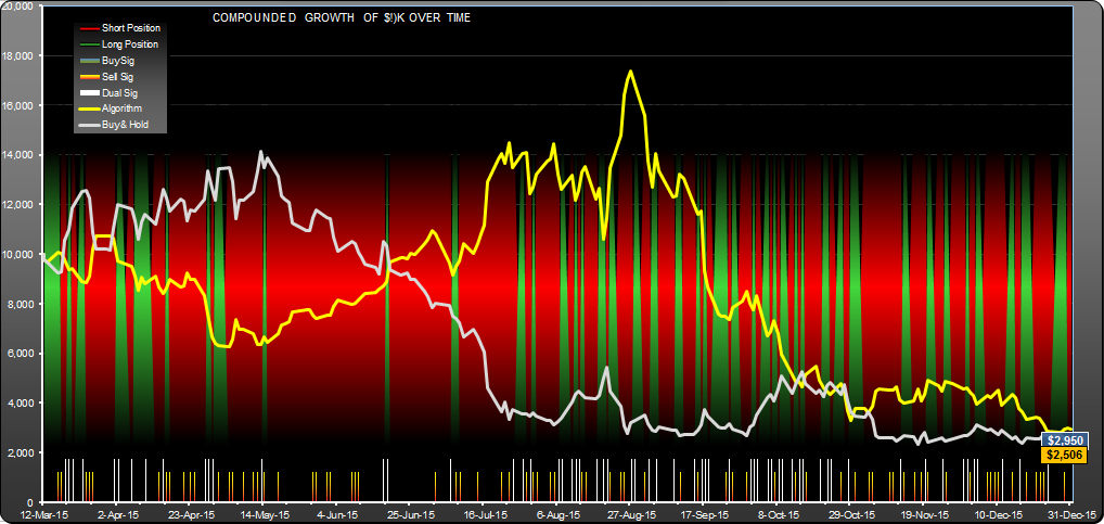
This is an interesting AAPL trading strategy for the period 12/12/80 through 7/31/15, which would have generated $8,521,705,763 in profits from $10,000 initial investment. Buy and hold would have generated $2,744,894 in profit in the same period. The cover and buy signals were generated when the stock price dropped 37.77% below the 20 month exponential moving average. Short and sell signals were generated when the price dropped 30.01% below the previous month’s high. Positions alternate between long and short. There were a total of 44 buy signals and 44 sell signals, you can see them at the bottom of the equity curve as vertical lines:

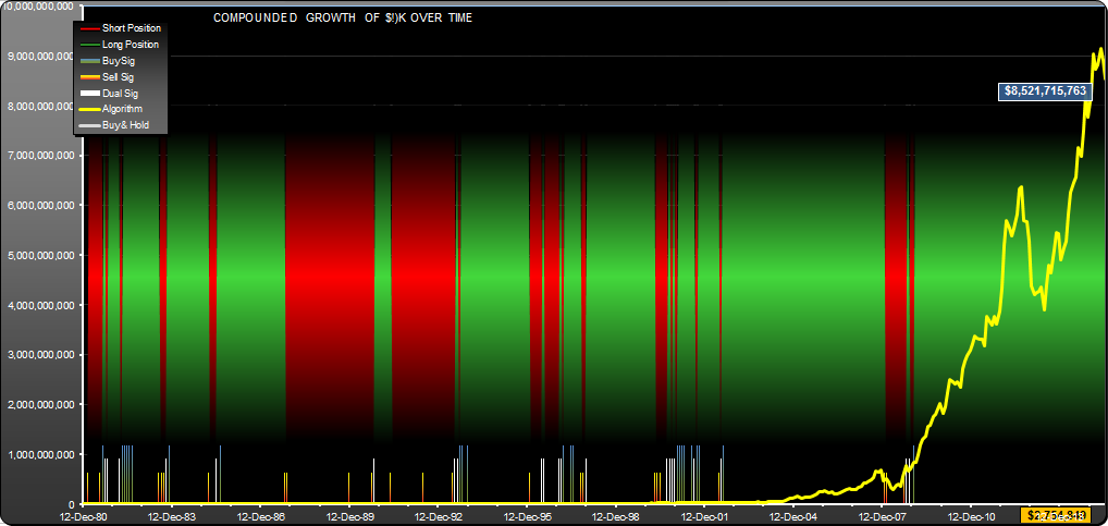
Blue/green lines are buy signals(23), red/yellow lines are sell signals (23) and white lines are dual signals (21). A dual signal always leads to a trade, but a buy signal would only lead to a trade if you were short, and a sell signal would only lead to a trade if you were long. So you can see there was some nice reinforcement on the signals.

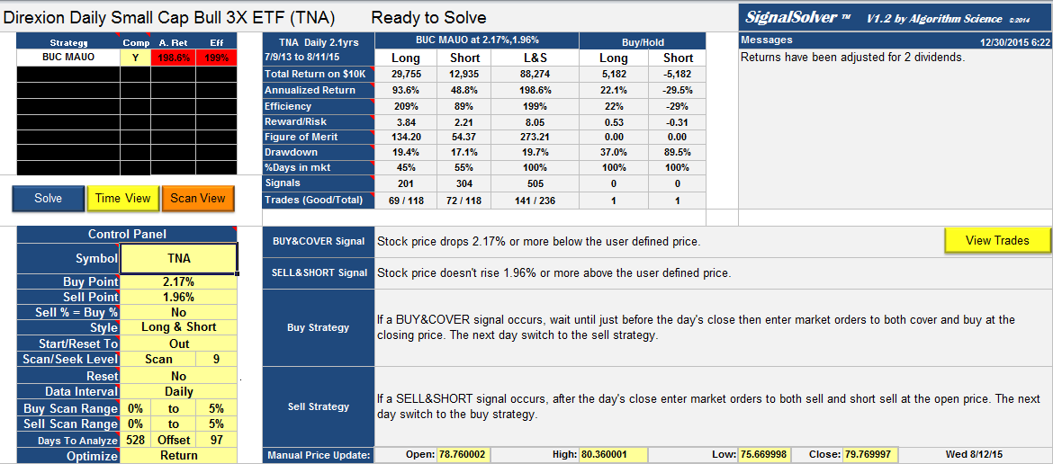
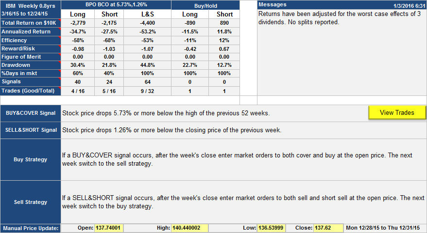
The AAPL trading strategy and its performance

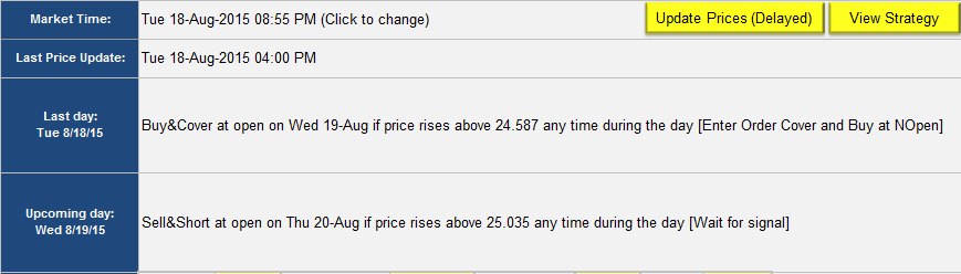
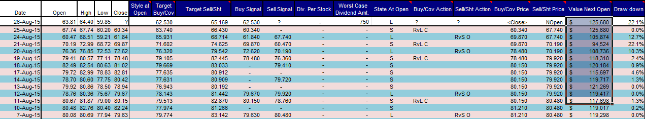
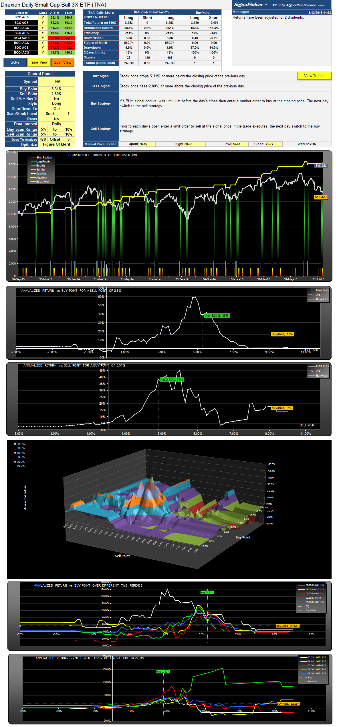
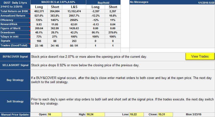
Selling/shorting was done at the next month’s open using market orders, while buying/covering was done when the signal arrived using limit orders. The green and red backgrounds behind the equity curve shows if you were long or short. The rules governing the strategy are shown in the performance table below. Signals are straightforward and response to signals is also simple.

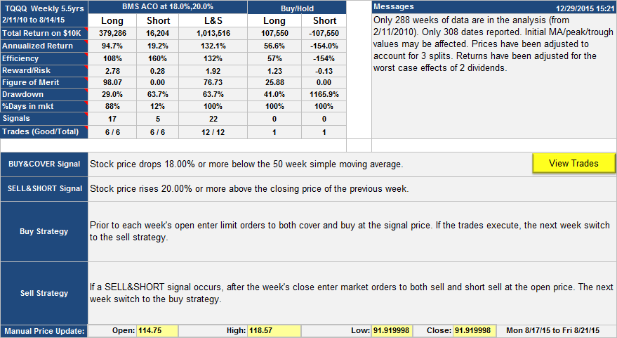
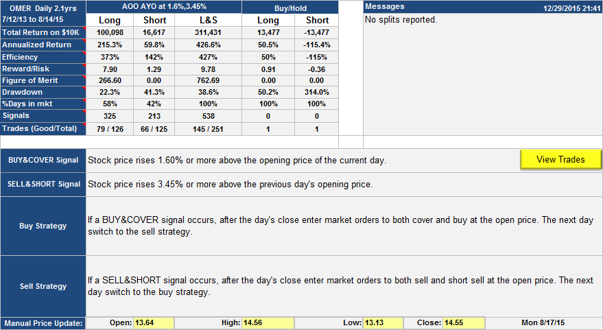
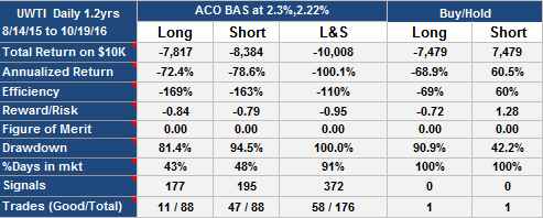
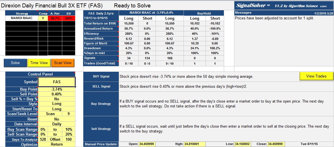
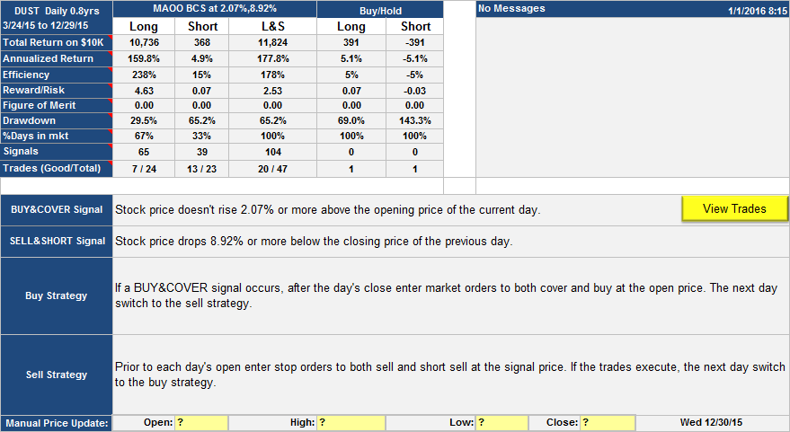
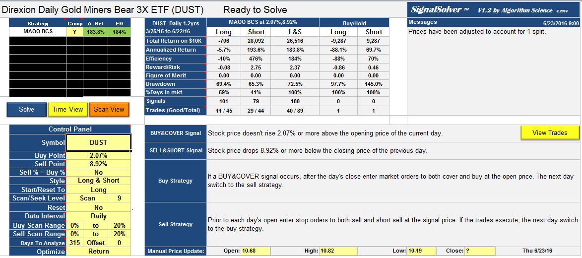
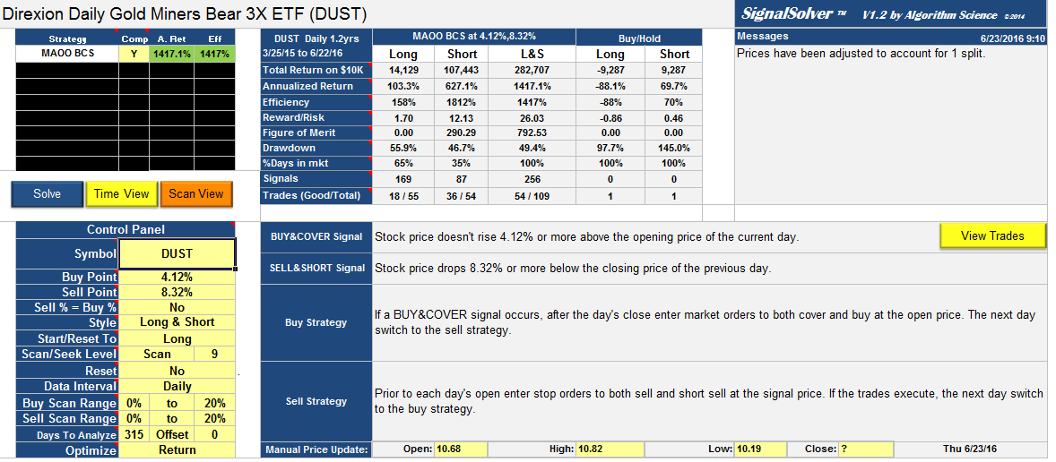
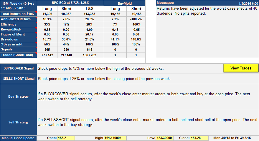
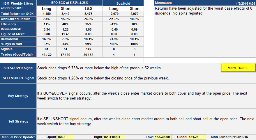
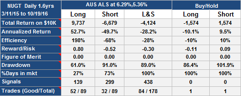
Had you been lucky enough to have been following this AAPL trading  strategy, you would have needed to check in on it only once a month before the monthly open to place orders, a few minutes work. Only 39 of the orders placed actually executed as you can see from the Performance Table:

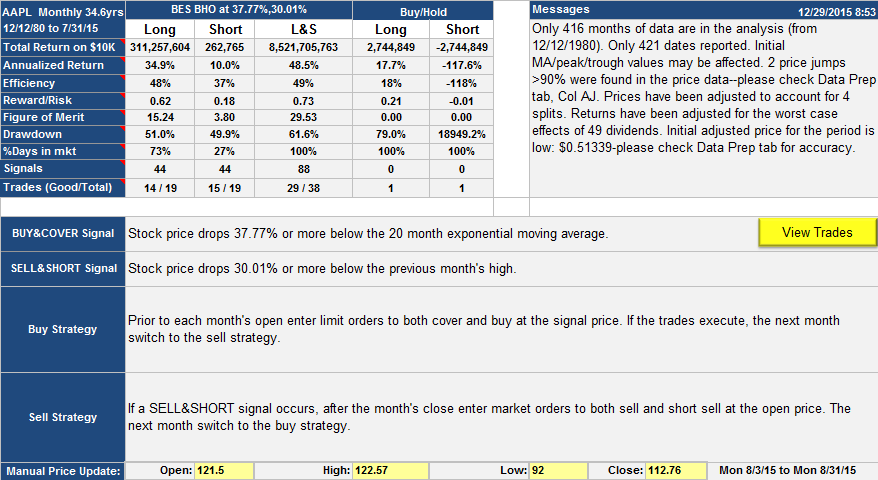
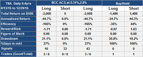
A few points about the Performance Table; In the Messages section you can see some warnings about the way the stock price moved. SignalSolver warns you about price jumps so you can check them out. In this particular case the jumps were for real–one drop in Oct 1987 (Black Monday), the other a drop in Sept 2000 as the dot com bubble burst.

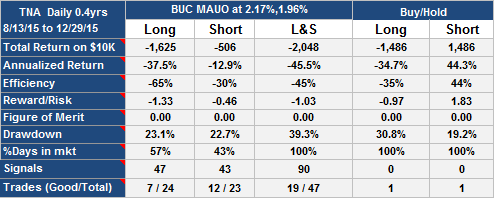
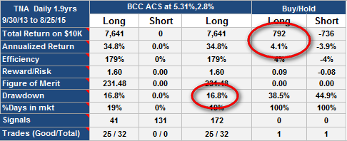
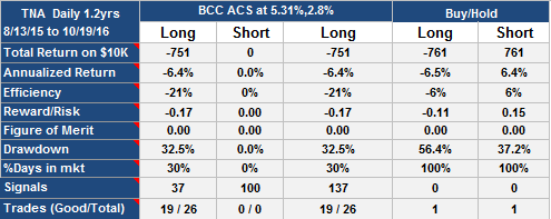
The Performance Table also tells you how you would have fared if you had only played the long side (i.e. never gone short), or if you you had played the short side and never gone long. Clearly, playing both long and short (the L&S Column) sides was a better strategy in this instance, however you would have lost everything if the buy and sell points were not exactly as described.

Drawdown is the most you could have lost if you had entered a strategy at the worst possible time and then stopped using the strategy at the worst possible time. Notice the drawdown for the trading strategy was 61.6%. This may seem extreme, until you look at buy and hold drawdown of 79%.

Efficiency (relevant only for the long only and short only sides of the trading strategy) tells you the annualized return if you had invested at the same rate when you were not holding AAPL long or short. Its the annualized return divided by the % of time in the market. Reward/risk is the annualized return divided by the drawdown plus a 5% offset.

Figure of Merit is what the optimizing backtester uses to grade each of the algorithms. It can be set up to look for a rich variety of attributes like total return, drawdown or efficiency. In this instance we compared around 47,000 algorithms with about 13 million backtests optimizing min quartus return (see below).

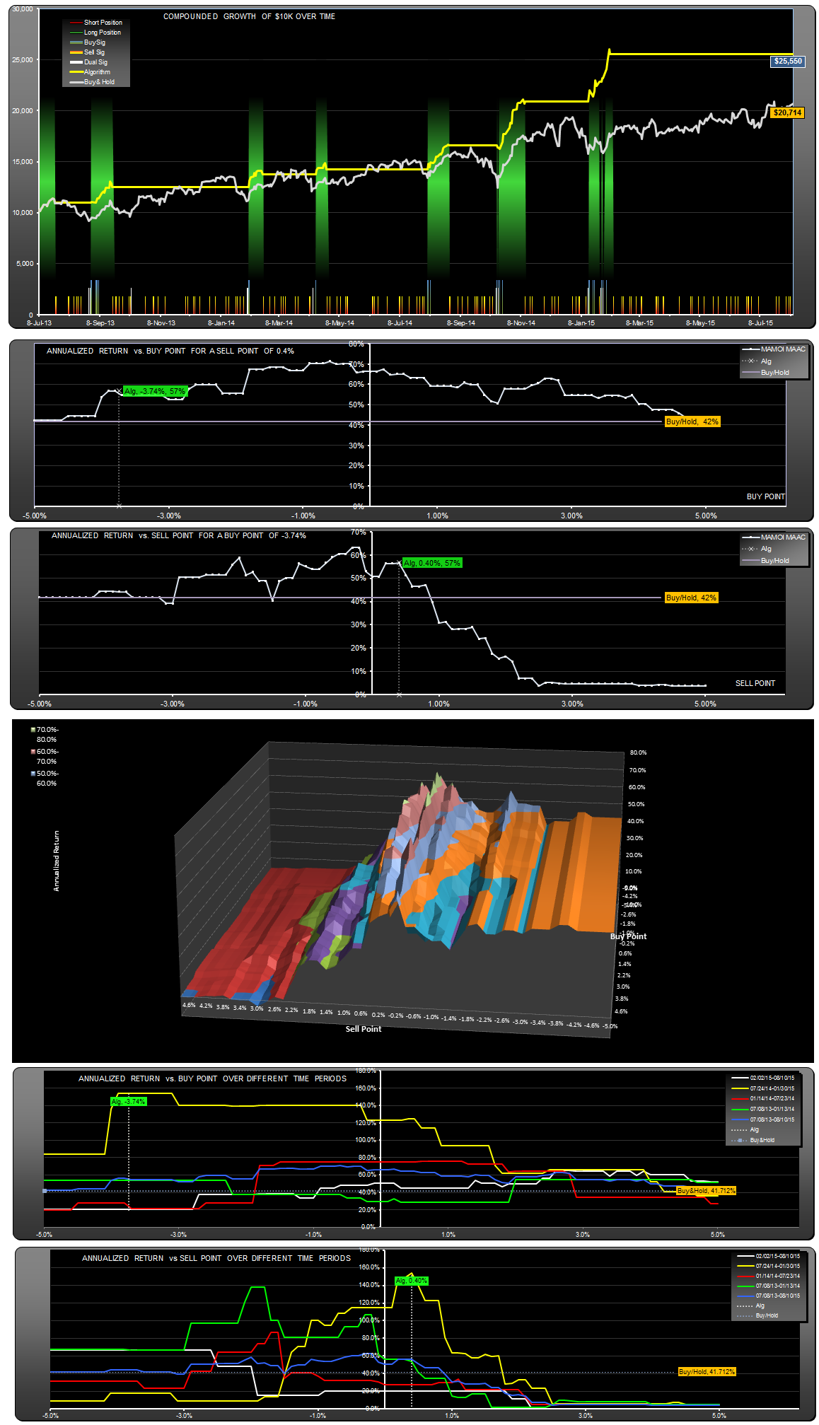
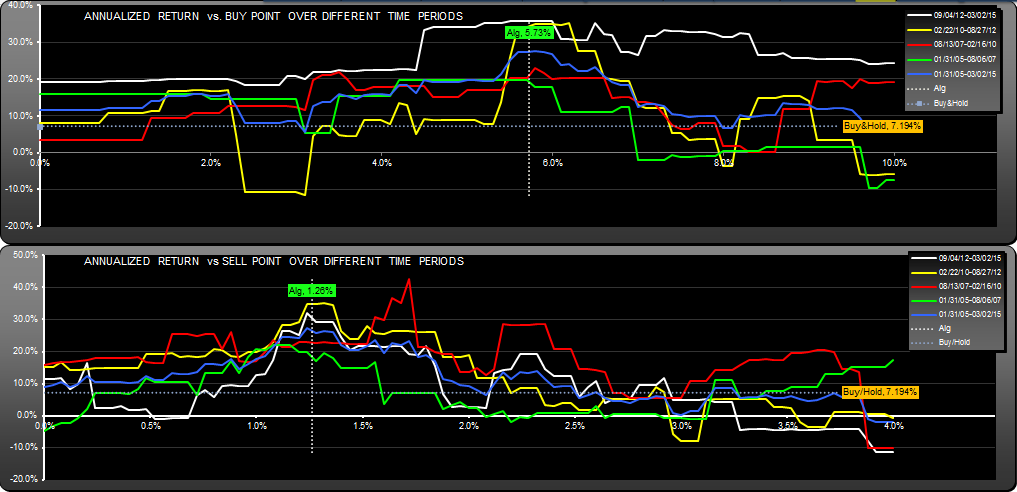
The effect of parameter changes on return

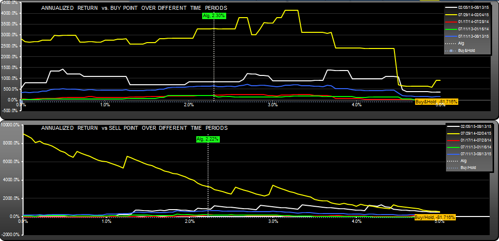
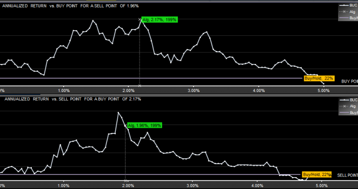
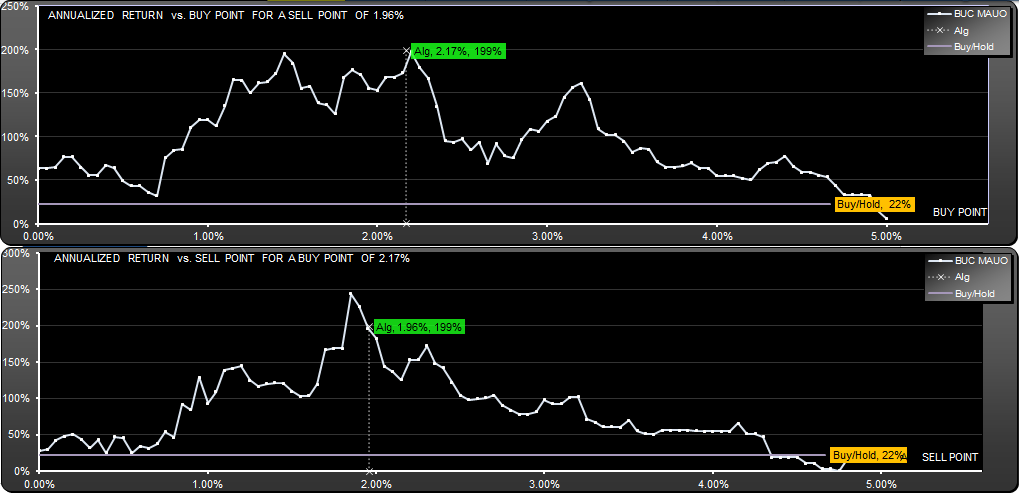
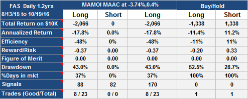
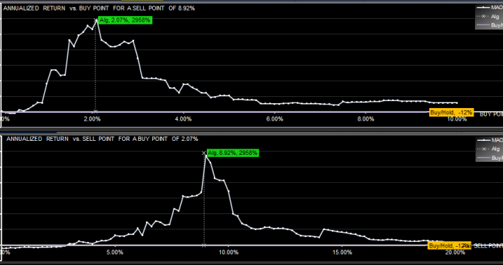
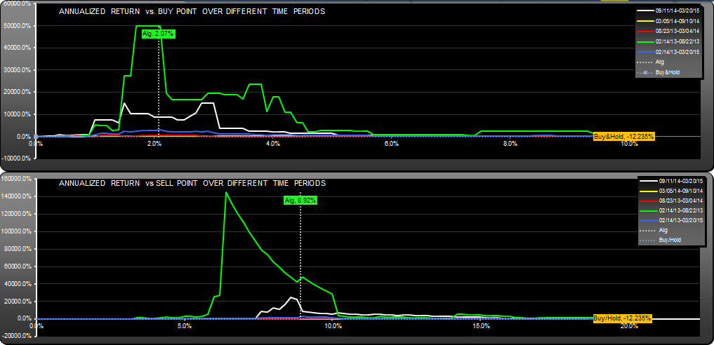
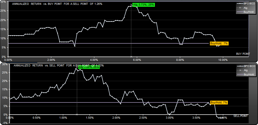
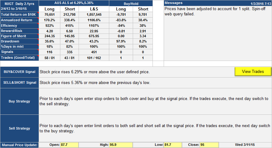
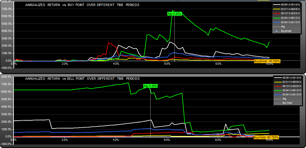
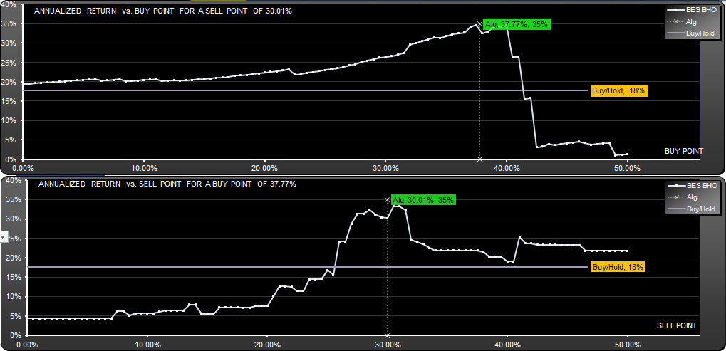
Now we’ll take a closer look at the buy and sell parameters. Remember the strategy–buy if price drops 37.77% below the 20 month exponential moving average, sell if price drops 30.01% below the high of the previous month. Well, you need to look at the effect on return if you change those percentages. For that we look at the Scan Charts. First, the scan chart for Long and Short style.

AAPL.M2 Scan LS

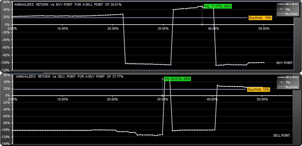
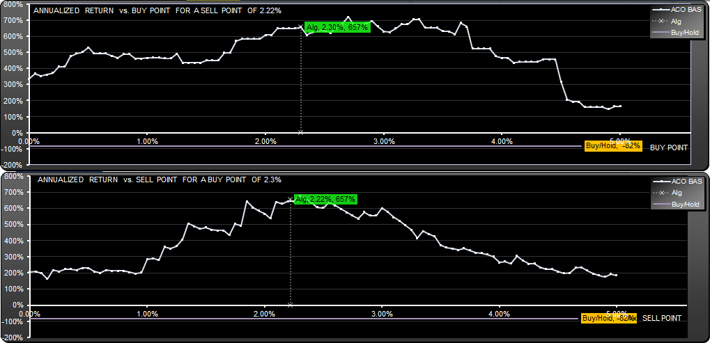
This shows that the profitable sell point range was very tight, between 30 and 32 %. Outside of this was a total loss. When you compare this with the scan for the Long only strategy, shown below, you can see the extreme downside risk of short selling a stock like AAPL. This makes the Long and Short strategy too risky to consider further, however the Long only strategy, with its 35% annualized return is still interesting, so we shall focus on that. Here it is:-

AAPL.M2 Table Long

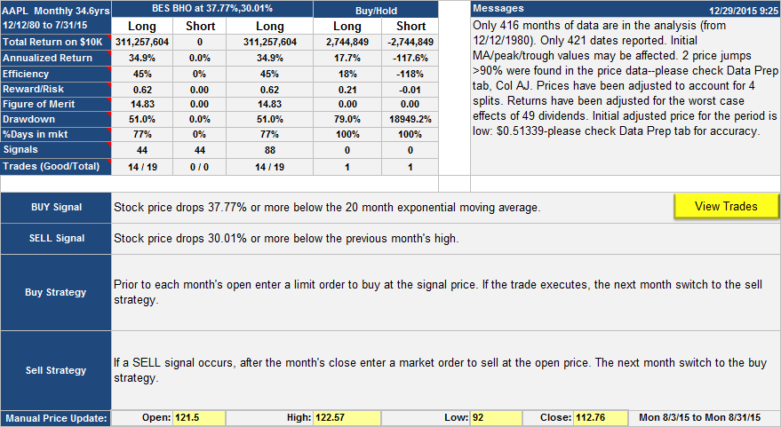
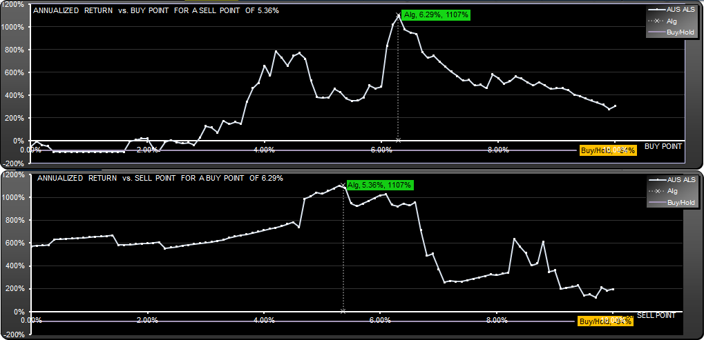
and here is the scan result:

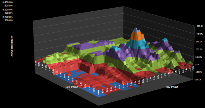
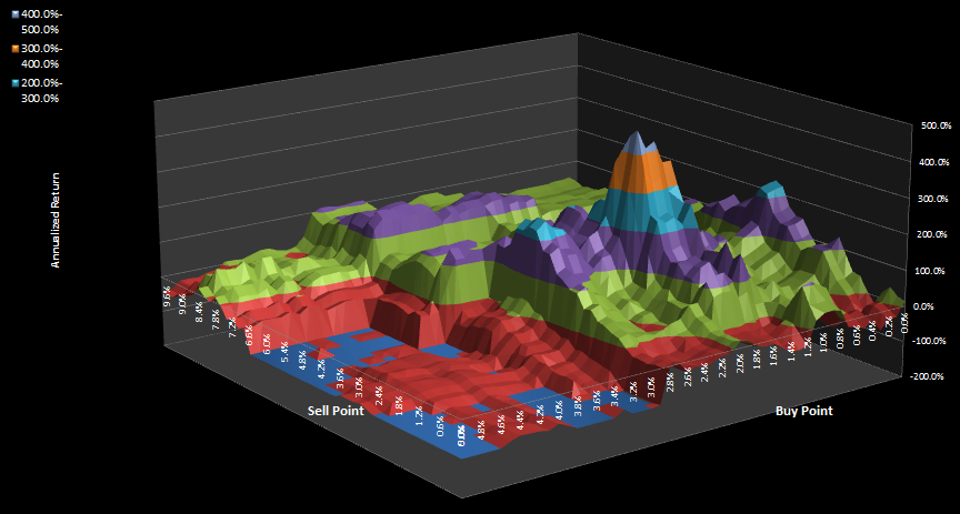
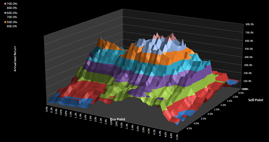
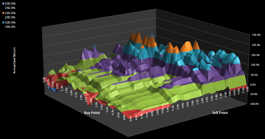
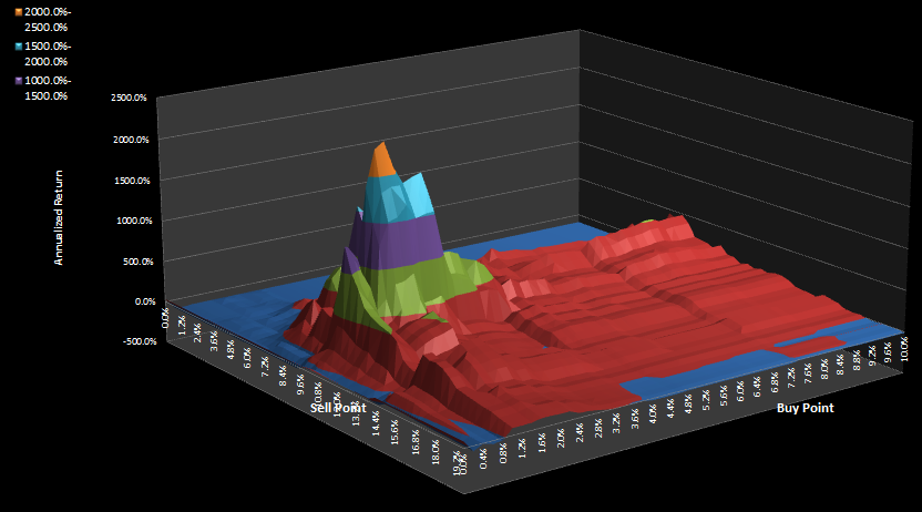
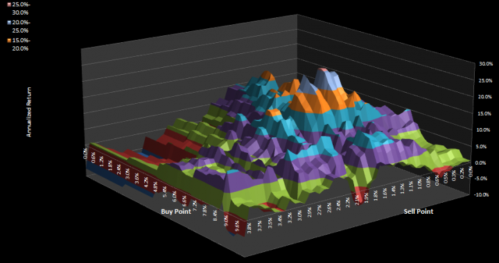
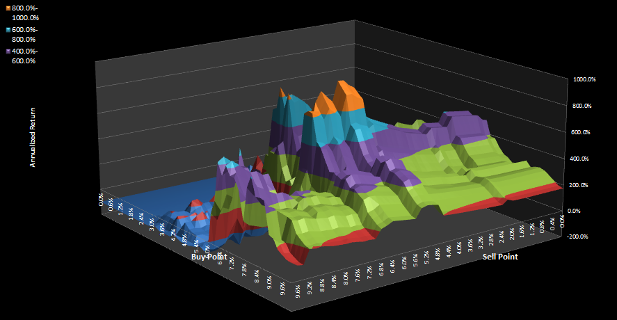
This is a much nicer scan result than the Long & Short strategy result. Focusing on the Long only scan, you can see from the top scan that if you had got the sell percentage right but used a buy point of 42%, then you would have done much worse. Similarly, if you had got the buy percentage right but used a sell percentage of 20%, again you would have reduced the profits considerably. On the positive side, if your sell point was 30.01%, you would have done better than buy hold for any buy percentage below 41.5%. Or, if your buy % was 37.77%, then you would have done better than buy-hold for or any buy % greater than 26%. But that’s not the whole picture. You can plot returns for every value of buy and sell point in the form of a surface plot:

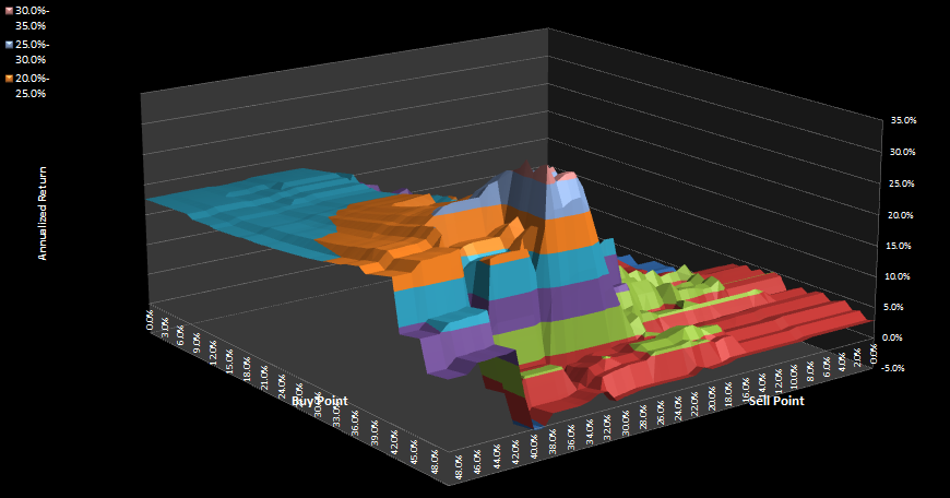
If you run SignalSolver, you can spin the surface plot around to take a good look for areas of low return were you could have got into trouble. The higher the hill, the more return you would have made if you were using those buy and sell points. You wanted to be high on the “hill” but not close to any cliffs as they imply risk.

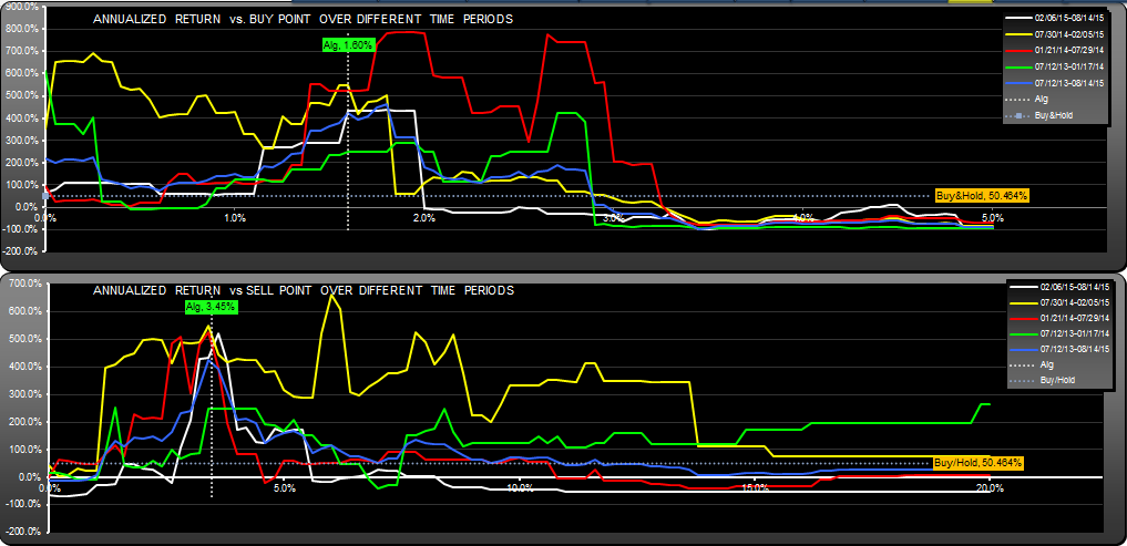
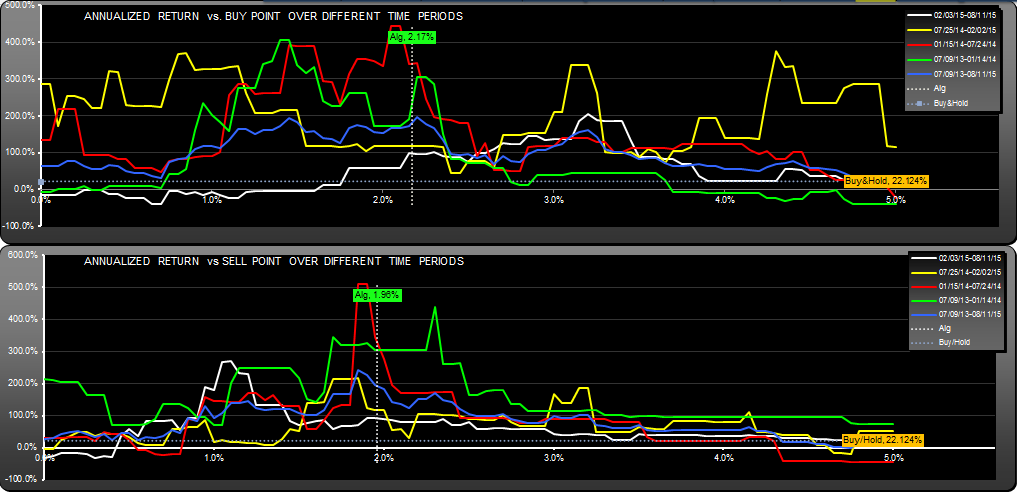
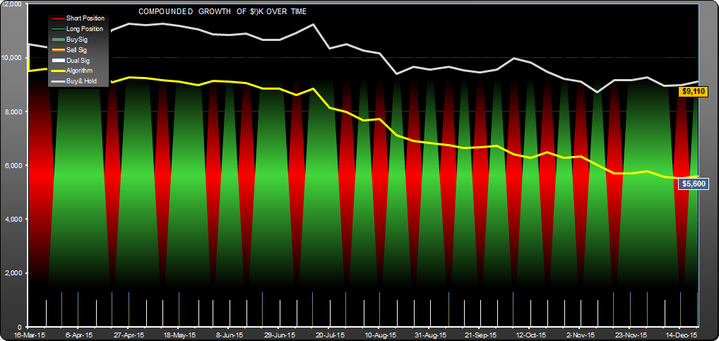
The next question is how did returns change over time for different buy-sell points? To answer this we use the “Life” Scan Chart:

AAPL.M2 Life Long

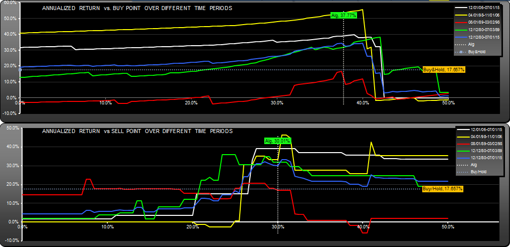
The Life scans are expanded views of the Scan Chart, in fact the blue line is exactly the same graph. The other lines show how the returns changed with buy and sell parameters for other time periods. Each time period is one quarter of the entire data set which happens to be 104 months (8.66 years) for this analysis. We call this a “quartus” (latin for one fourth) to avoid the ambiguous term “quarter”.

The trading strategy was found by setting up the SignalSolver backtester to search for the algorithm with the best “worst quartus”. Effectively, its looking for space under the Life scans. In this case, the annualized return for the worst quartus was 17% for the red period (8/1/89-3/2/98) while the best quartus was 53% ann. return for the yellow period (4/1/98-11/01/06). So while the return is nowhere near the highest returns I have found for an AAPL trading strategy, I think the (long only) strategy has better consistency and less sensitivity to the buy/sell parameters.

Note that the backtests assume a transaction fee of $7 per trade and slippage of 0%.

Here is the list of trades for the long side: AAPL.M2 Trades Long.

Andrew

Please note that there were errors in the original posting related to the short side of this algorithm. These have now been corrected (12/29/2015)
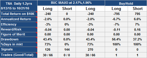
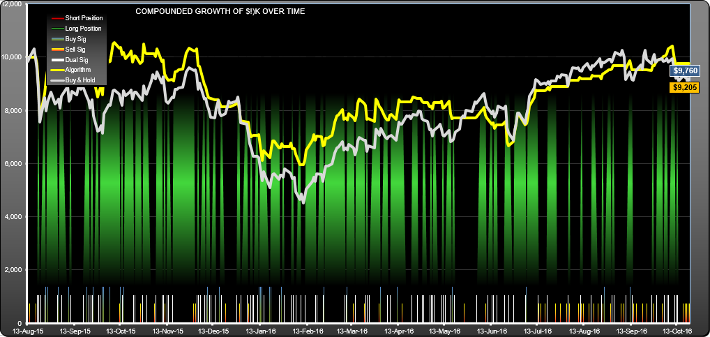
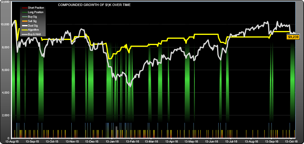
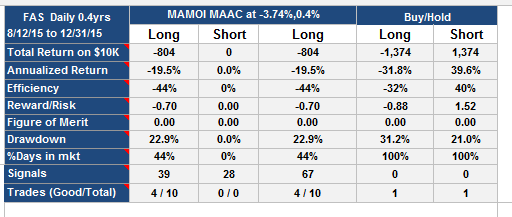
Update 10-20-2016

Strategy has followed buy-hold, losing about 4.8% since publication

UWTI Trading Strategy (daily)

This UWTI trading strategy would have returned $676,147 for $10K outlay over a 2 year period. It was a very straightforward strategy with simple maintainence, once a day you would have put in either market orders to cover and buy or stop orders to sell and short before the open. This is another result discovered by optimizing minimum quartus returns, a SignalSolver backest optimization technique. A quartus is one-fourth of the data and we look for algorithms which give the best minimum return of all four quartus results. In this case it was 206% annualized for the period June 2013 to Jan 2014. It happened to be the fourth best result found for this particular scan of 500 algorithms but I chose it because the drawdown was significantly better than for the other 3 (30.7% vs 55% for short-hold).

Results for this strategy were not consistent, most of the gains were made in the period June 2014 to Feb 2015.

UWTI-D Table

UWTI-D Equity

UWTI-D Life

UWTI-D Scan

UWTI-D Surface

A list of trades in spreadsheet format: UWTI-D Trades

Update 12-30-2015:

The above analysis has been corrected for a miscalculation of the short-side return of this algorithm.

UWTI-D Table Update1

UWTI-D Equity Update1

Update 10-20-2016

This algorithm turned a complete loss:

UWTI Trading Strategy Update 10-20-2016

UWTI Trading Strategy Update 10-20-2016

TNA Trading Strategy (Daily)

In contrast to yesterday’s TNA trading strategy optimized for low drawdown, this one is optimized for minimum quartus annual return, a new feature of SignalSolver. A quartus is one quarter of the data, 132 days in this instance, and the minimum return was 99% annualized for the most recent quartus Feb 3 to Aug 11th 2015.

You can see how quartus annualized returns fluctuate with buy/sell parameters from the lifetime graphs. Note that this algorithm took both long and short positions–when you were not long, you were short. I have no idea how or why this kind of algorithm works–you would think the buy and sell signals are so similar that it would give more random returns, but you can see from the surface plot that the results are positive for most of the parameter space.

The “user defined price” was found by averaging the previous day’s high, the previous day’s low and the current day’s open price. Buying and selling was done at the daily close or next day’s open.

TNA-D Table

TNA-D Equity

TNA-D Life

TNA-D Scan

TNA-D Surface


List of trades in .xlsx format:  TNA-D Trades


Update 8/26/2015

Trades since the original backtest endpoint on 8/11/2015:

TNA.D2 Update 8-26-15

Update 12/30/2015

The above analyses have been corrected for an error in the short-side returns. Overall gain of the original erroneous post was $104,971

Here are the updates for 12/30/15. The algorithm peaked around Oct 13th and now appears to be failing:

TNA-D Equity Update 12-30-15

TNA-D Table Update 12-30-15

Update 10/20/2016

A bit of an improvement:

TNA Trading Strategy Update Oct 2016 Equity

TNA Trading Strategy Update Oct 2016 Equity

TNA Trading Strategy

Another low drawdown trading strategy-TNA Direxion Daily Small Cap Bull 3X

In the same vein as yesterday's FAS analysis, here is a low drawdown trading strategy for TNA, with daily intervention. Prasad had asked me to search for low drawdown strategies for a few of the triple leveraged ETFs, this being one of them. As with FAS, the algorithm was found by optimizing the SignalSolver backtest engine for drawdown (100% weighting), with a min QA return weight of 50% thrown in to get rid of all the zero trades-zero return hits. Period of the analysis was 1.9 years.

Again, the result had a low time in the market (18%), low drawdown (4.9%) and an annualized return which, while modest (38%), was better than the underlying ETF.

Andrew

TNA.D


Update 8-26-15

As per the table below, you can see the drawdown has jumped up to 16.8%. On the positive side, the differential in performance of the algorithm vs. the underlying TNA stock has grown. 

TNA.D Update 8-26-15


Update 12-30-2015

This algorithm peaked close to the day of publication, and has not done well since then:

TNA-D Low Drawdown Update 12-30-15 Equity

TNA-D Low Drawdown Update 12-30-15

Update 10-20-2016

Slight improvement over last update:

TNA Trading System Update 10-20-2016

TNA Trading System Update 10-20-2016

FAS (daily)

FAS (Direxion Daily Financial Bull 3X ETF) trading strategy with low drawdown

This is one of the triple leveraged funds which Prasad had asked me to come up with a low drawdown trading strategy for,  I'll be looking at the others soon. You can set up SignalSolver to optimize for low drawdown. The way you do that is by setting up the Figure of Merit parameters to look for low drawdown, however you need to fold return into the picture, otherwise it simply comes up with algorithms that don't trade and have zero drawdown. In this instance I set the FOM parameters to be Total Return (25%), drawdown (100%) and Min Quartus Return of (25%). The data is divided into four quartus's, so including Min Quartus Return gives more consistent returns than just including Total Return. 

A few things to note about this result. The drawdown (the worst case loss you would have suffered if you had entered and exited the strategy once) was 4.5% compared with the underlying stock's drawdown of 24%, and the total return beat the return of the underlying stock (56.7% annualized vs. 41.7%).  Its a long-only strategy. If you had shorted instead of exiting, the drawdown was close to 30%. The trading strategy was also very efficient, that is, the returns were good given the small amount of time (20%) you were in the market. If you could have invested at the same rate of return during the 'out' periods, you would be talking about a 288% annualized return (a figure I call Efficiency).

The trading strategy didn't trade frequently, nor was it particularly consistent in its results, as you can see from the last two graphs below. Also, its not particularly stable with respect to the buy and sell point percentages as you can see from the surface plot. None of these factors suggest a strategy worth pursuing--its really just a curiosity, a demonstration that you can find low drawdown strategies that worked if you look for them.  

One last point of clarification, the buy signal is a negative percentage (-3.74%) with respect to the reference (the 50 day simple MA). If you were waiting for a buy signal and the 50 day SMA at the previous daily close was at $100, then the buy signal would occur if the stock price failed to rise above $96.26, assuming no sell signal. Buying was done at the subsequent open, selling at the close on the day of the sell signal.

Andrew

FAS-D 4.5 Corrected Table

FAS.D 4.5 DD Correction

Post has been corrected 1-2-15 for an error in short-hold calculation.

Update 1-2-16

Low drawdown did not last, but did better than buy-hold:

FAS-D1-1-16 Update Table

Update 10-20-2016

FAS Trading Strategy (Daily) Update 10-20-2016

FAS Trading Strategy (Daily) Update 10-20-2016

DUST Daily Trading Strategy

This trading strategy is for stock symbol DUST the Direxion Daily Gold Miners Bear 3X ETF. It is the complementary stock to NUGT which I analyzed last week. Its not hard to find strategies which would have exploited the intense volatility of this kind of security, if you have access to an optimizing backtester. The strategy presented here gave good returns and reward-risk. Most of the returns were in the period Feb 2013 to Nov 2013, in which period $10K would have turned into $750,000. By Nov 2014, the investment compounded would have been worth $5m and since then until now (Mar 2015) it would have turned into $13m (list of trades). It will be interesting to see if the growth continues. I wouldn't expect it to, given the inconsistent performance, but you never know. In contrast, buy and hold lost 20% over the same period.

The strategy itself can be read off from the table below, its a daily trading strategy which means that you would have had to attend to it on a daily basis. It would have taken a few minutes a day to work out the signals and enter the orders. Note that you would have to short the stock if you were long and a sell signal showed up. Using NUGT as the shorting vehicle would have given different results.

Just a reminder; don't expect to implement this kind of algorithm and get similar results. I'll be tracking it on paper and give updates, so watch this space.

This strategy was corrected 1/1/16 to account for an error in the short-side returns.


Update 1/1/16

This strategy did OK after publication. For the period 3/24/15 to 12/29/15 the equity and stats are shown below:


DUST-D Equity 1-1-16

DUST-D Table 1-1-16

The optimum buy and sell points for this period would have been 4.13% and 8.45% (returning $66,246).

Update 6/23/2016


Since the original posting in March 2016, this strategy has returned 183% annual return, but in an extremely choppy fashion:

DUST-D Update 6-23-16 TimeDUST-D Update 6-23-16 Table

The optimum buy point over this period was 4.12%, with a sell point of 8.32%. The results for this optimization are shown in the table below. Its odd how the optimum buy point was almost exactly twice that of the original optimization, not the first time I have seen this happen.

DUST-D Update 6-23-16 Table Opt

DUST-D Update 6-23-16 Time Opt

Update 10/20/2016


Performance has deteriorated somewhat:

DUST Trading Strategy (Daily) Update 10-20-2016

DUST Trading Strategy (Daily) Update 10-20-2016


IBM Trading Strategy (Weekly)

This IBM trading strategy made 11x the total returns (4x the annualized return) of the underlying stock with half the drawdown. The backtest period was 10years. The strategy itself (see table below) was straightforward with both buy and sell signals triggered by falling prices. The buy signal keyed off the 52 week high while the sell signal keyed off the closing price of the previous week. All buying and selling was done at the weekly open. It turns out that 225 out of 528 weeks were dual signal days, this often led to periods where a buy weeks alternated with sell weeks (see list of trades in excel format). Ignoring dual signal days would have led to very low gains, so the alternating strategy must have worked somehow.

The strategy had a buy bias, there were 141 days with just a buy signal and 55 days with just a sell signal. Since the underlying stock seems to be downwardly trending, this bias may work negatively if the downtrend continues. We shall see.

The backtest assumes a commission of $7 per trade.


Update 1-3-16

This this strategy turned out to be a dramatic failure. Here are the updated table and equity curves:

IBM-W Equity1-3-16

IBM-W Table 1-3-16

Update 1-3-16

Still a dramatic failure, but less so:

IBM Trading Strategy (Weekly) Update 10-20-2016

IBM Trading Strategy (Weekly) Update 10-20-2016


NUGT Trading Strategy (Daily)

Original Post March 12th 2015

Please note, this post was corrected 1-3-16 to account for a short-side error in the original calculations. Apologies for this.

This NUGT trading strategy (Direxion Daily Gold Miners Bull 3X ETF) gave a theoretical $1.8 million profit for a $10K initial investment over 2.1 years. The trading strategy required once a day attention. Signals were triggered by rising prices on both the buy and sell side. The buy side reference was 1.0629 times the average of the previous day high, the previous day low and the current day open. You would need to calculate it every day after the open and then put in the buy and cover orders, if you were short. On a few occasions this meant buying at the open price, but usually there was time to get the stop orders in.

The sell side target was a bit simpler, 1.0536 times the previous days low. You could enter the sell and short limit orders after each close, if you were long.

There is a Bear version of this fund, the Direxion Daily Gold Miners Bear 3X ETF (DUST), however the results would have been different if you had used it for the short side.

Here is the list of trades.


Update 1-3-16

The algorithm peaked at the end of Aug 2015:

NUGT.D Equity 1-3-16

Update 10-20-2016

Since it peaked at the end of Aug 2015 the algorithm has not recovered:

NUGT Trading Strategy (Daily) Update 10-20-2016

NUGT Trading Strategy (Daily) Update 10-20-2016