Bitcoin trading strategy using SignalSolver Sentiment

Bitcoin Trading Strategy using SignalSolver Sentiment

This trading strategy for Bitcoin uses SignalSolver Sentiment to generate trading signals. It is currently showing a 22% drawdown, but it has been a good performer overall. Sentiment on any given day is determined by backtesting up to that day, selecting the top algorithms and evaluating the ratio of long to short positions. Sentiment (percentage bullish) is shown as a blue bar-chart on the graph. Trading is performed subsequent to the Sentiment crossing a threshold value.

The Buy and Sell thresholds for this simulation (green and red lines on the time graph) used an adaptive technique every cycle to determine the optimum values, with the constraints Buy+Sell=100% and Buy>Sell. The optimum thresholds settled down pretty quickly to Buy=55% and Sell=45%. Return was $67,966 since 1/1/21 for a $10,000 outlay (CAGR 0f 273%), with Risk-Reward about 680 times that for Short-hold. The simulations assume the ability to both long and short the security, but the table includes both the Long and Short returns

Bitcoin trading using SignalSolver Sentiment with adaptive symmetric thresholds

Bitcoin trading using SignalSolver Sentiment with adaptive symmetric thresholds

In selecting a threshold strategy, you couldn't get into too much trouble since the other two common threshold strategies also showed a profit. Using an adaptive threshold with the Buy=Sell constraint applied returned $25,206 (123% CAGR)--

Bitcoin trading using SignalSolver Sentiment, adaptive equal thresholds

Bitcoin trading using SignalSolver Sentiment, adaptive equal thresholds

Finally applying a simple constant 50% threshold also worked well, returning $40,640 (183% CAGR).  From this image you can view the entire threshold surface, which is  what we like to see--a solid looking structure.

Bitcoin trading using SignalSolver Sentiment with a fixed 50% threshold

Bitcoin trading using SignalSolver Sentiment with a fixed 50% threshold

Settings are shown below:

SignalSolver settings for the Bitcoin Sentiment runs

SignalSolver settings for the Bitcoin Sentiment runs

These are the same settings we used for TQQQ with the only change being that we (somewhat arbitrarily) increased the number of algorithms to 21 (from 5 for TQQQ).  Only OHLC prices and short period (10 day) SMAs and EMAs are used in the backtests.

As with all Sentiment runs, out-of-sample walk-forward simulation is used. Sentiment is determined for a particular day by using the backtester on prior data, in this case using the ratio of the top 21 algorithms' long (bullish) to short (bearish) state. When the sentiment crosses the threshold in either direction, a trade is performed appropriately. In the case of Bitcoin, OHLC prices run from midnight to midnight.

TQQQ

AAPL signals prove versatile

AAPL signals prove versatile

Work on TQQQ, FNGU, NFLX and many others


The SignalSolver Sentiment indicator is calculated by aggregating multiple algorithm sentiments. The Sentiment technical indicator has a value between 0% (completely bearish) to 100% (completely bullish). Intuitively, you would think that a 50% threshold would be the best threshold value from which to generate buy and sell signals, and often this is the case. However, in the case of AAPL, the overall best Buy=Sell threshold (for the settings we are using) has been 85%. The result is shown below in the "L&S" column of the table:

AAPL performance using an 85% threshold

AAPL performance using an 85% threshold

The buy/sell signals generated by this algorithm have shown surprising versatility. Below are shown images showing the result of using the AAPL signals for AMZN, FB, FNGU, GOOG, MSFT, NFLX, NVDA, QQQ, TECL and TQQQ. In each case the result was better than both buy-hold and short-hold, often by an enormous margin.

The AAPL 85% Threshold

Success at using Sentiment to signal trades comes down to finding the best threshold to use. There are always values for the buy and sell threshold that generate equal or better returns than both buy-hold and short-hold. But you can only know these values retrospectively.

There was no way to predict that an 85% threshold would be optimum. However we can simulate (or run live) using an adaptive thresholds where the program optimizes the thresholds daily as you go along. When using this method, (as you might do in reality) the Buy=Sell constrained threshold was in the 80-90% range from Sept 2020 to Aug 2021 but then became unstable, with declining returns.

AAPL signal performance using adaptive threshold with constraint Buy=Sell

AAPL signal performance using adaptive threshold with constraint Buy=Sell

The threshold surface (shown below) is a very nice solid structure yielding a positive return for all constant values of threshold except the extreme edges. Notably, 50/50 yielded a return of twice that of buy-hold. The Buy>Sell adaptive threshold (also shown below) gave a better return than the Buy=Sell adaptive threshold, Here we optimize the thresholds every cycle as before.

AAPL Result using adaptive threshold with Buy>Sell constraint

AAPL Result using adaptive threshold with Buy>Sell constraint

Comparing the two results, you can see that when the Buy=Sell constraint is applied, the adaptive threshold appears to oscillate between the optimum buy threshold region and the optimum sell threshold region.

TQQQ trading strategy result

TQQQ Trading Strategy using SignalSolver Sentiment

TQQQ Trading Strategy using SignalSolver Sentiment

Post Updated June 29th 2022

This trading strategy for TQQQ uses SignalSolver Sentiment to generate trading signals.

We are updating the original post using improved settings. Two settings have been changed:

  1. The new post uses a Seek level of 4 instead of 2. So more algorithms are explored (although it takes a little longer)
  2. "A" suffix algorithms (those which buy and sell on the same day) have been excluded

The combined effect of these changes was to double the annualized return from 213% to 425%

Showing sentiment dashboard for the TQQQ run

Trading TQQQ using SignalSolver Sentiment would have yielded 425% annual return

50% Threshold is still the optimum, as you can see from the threshold surface. Additionally, this Sentiment run is 17 trading days further along than the Original Post, in which time the return has increased another 20% or so.

Trading FNGU using TQQQ signals

The signals generated by TQQQ Sentiment have been found to work well for FNGU (and many other symbols also):

Showing the Sentiment Dashboard for FNGU

When traded using TQQQ Sentiment signals, FNGU would have yielded 961% annualized return

This is the same Sentiment profile as generated by TQQQ, but the signals are used to trade FNGU (easy to simulate in SignalSolver, just change the symbol). Here the annualized return was 961%.

The settings for these runs are exactly the same as the Original Post (click below), with the two changes noted above.

Click to view the original post Dated June 2nd 2022


This TQQQ trading strategy using SignalSolver Sentiment gave 213% annualized return for the period Jan 4th 2021 to June 2nd 2022. The sentiment threshold was set to 50% for the entire period.

Sentiment run for TQQQ showing 213% Annualized Return

TQQQ Sentiment Run showing 213% Annualized Return. Notice good symmetry and structure on the Threshold Surface.

Settings are shown below:

Settings Tab settings

Settings Tab

Notice that only OHLC prices and short period (10 day) SMAs and EMAs are used in the backtests.

Below are shown the Report Tab settings, notably 240 days of data were used for the backtests, and only percentage band was used (PB).  As with all Sentiment runs, out-of-sample walk-forward simulation is used. Sentiment is determined for a particular day by using the backtester on prior data, using the top 5 algorithms’ long or short state. If the sentiment crosses the 50% threshold in either direction, a trade is performed appropriately.

Report Tab Settings.

Report Tab Settings.

AAPL Trading System using SignalSolver Sentiment

AAPL Trading using SignalSolver Sentiment

AAPL trading using SignalSolver Sentiment

Using multiple algorithms to drive trading strategy

Original Post July 23 2021

AAPL Trading System using SignalSolver Sentiment

AAPL trading system using SignalSolver Sentiment

Methodology

Shown above is the simulated result of trading AAPL using SignalSolver Sentiment. The sentiment is shown as a blue area chart in the background. The equity curve for the strategy is shown in yellow, buy-hold equity in white. Sentiment is calculated each day after the close of business by assessing what percentage of the top 50 SignalSolver backtest algorithms are bullish. The buy and sell thresholds are fixed at 50% (red line) with bullish being above the threshold. A trade is executed at the next open whenever a change in sentiment is indicated, so the trade price is always out-of-sample from the backtest period which is fixed at 250 trading days. The simulation then walks forward to the next day, repetitively. Algorithms are re-parametrized every 10 trading days and flushed and refreshed every 50 trading days. For more information on methodology, please see here.

Performance of simulated AAPL trading system using SignalSolver Sentiment

Performance of AAPL trading system using SignalSolver Sentiment

Performance

Trading on sentiment (L&S column above) performed around four times better in this simulation than buy-hold in terms of reward/risk, with final equity being around 3 times better for Long/Short trading of the signals and trading long only being about twice as good. In all cases, drawdown was lower for the sentiment trading than for buy-hold.

Below is shown the threshold surface for the equal buy/sell thresholds showing that annualized return (CAGR) is insensitive to threshold changes. The peak return is $26,863 at a threshold value of 83%.

Click here to see the SignalSolver settings for this strategy: AAPL Sentiment Settings

We now move into the paper-trading phase for this project. Updates will be shown below.

Updates

We tracked this algorithm with daily updates (up until Jan 4th 2022) here.

As of Jan 4th, (the time we stopped tracking it), here's how it looked:

AAPL performance for 50-50 thresholds

From July 16th 2021 (the time we started paper trading this algorithm) it had lost 12.4%. Not good.

What we could have done better

We should not have forced a 50% threshold. It worked fairly well until 11/30/21 when it reached a peak of $37,705, up from $32,323 or a gain of 16.6% (vs. 25% gain in the underlying stock). But let's look at what would have happened if we had allowed the thresholds to float:

Here we are allowing the buy and sell thresholds to float, with the stipulation that the buy threshold must be greater than the sell threshold and the buy and sell thresholds must add up to 100% (the Symmetric box is ticked). Also we have set, Optimize Every to re-optimize the thresholds every day (set to 1) and we use an Optimization Window of 252 trading days (1 calendar year). This gives a return between July 16th 2021 to Jan 4th 2022 of 33% (vs. just under 20% for buy-hold).

Hindsight is 20/20. When we made the decision to run with 50% thresholds (on July 15th 2021), the return of its algorithm since Jun 12th 2020 was higher than that for the floating thresholds--203% annualized vs. 160% annualized.

Back in July 2021 the constant 50% threshold algorithm (above) looked better than the adaptive threshold algorithm (below). Sentiment is shown in blue, algorithm in yellow and buy-hold in white.

AAPL adaptive threshold algorithm vs. buy-hold

The adaptive symmetrical threshold algorithm back in July 2021 when we started trading. Buy threshold is green, sell threshold in red. Part of the under-performance is due to threshold hunting at the start of the run. Ultimately this was the better strategy.

Plus, 50-50 thresholds have a certain hard-to-resist appeal. But given the fact that AAPL (and most of the other stocks we tracked) did better with a floating threshold, we have become wiser. Lets track this algorithm for a while and see what it does.

A quick word about the floating thresholds. A 76/24 threshold was established in mid September 2020. Shown below is what the backtest looked like in July 2021 using a constant 76/24 threshold right back to the June 12th 2020 sentiment run start date. It actually outperforms every constant equal threshold algorithm, so the clues were there. Had we stuck with the constant 76/24 thresholds, we would have netted a 36% profit from July 16th 2021 to Jan 4th 2022, an even better result than the floating thresholds.

AAPL backtest result July 2021 using symmetric 74% buy and 26% sell thresholds

AAPL Backtest result for using a constant 76% buy threshold and 24% sell threshold at the decision point of 7/16/21. It is a better result than the 50/50 threshold and we could have moved forward with this strategy with good results.


Update 7/7/2022

The adaptive threshold used above did not work out, losing 14% since the last update on 2/4/2022. Disappointing that it did not go bearish since the last update.

FAS trading simulation

FAS trading strategy using SignalSolver Sentiment

FAS trading using SignalSolver Sentiment

A sentiment driven trading strategy with adaptive thresholds

Methodology

Sentiment is usually based on a consensus of opinions of expert humans. In contrast, SignalSolver sentiment is the consensus opinion of multiple backtest algorithms. This is a trading strategy for the FAS financials triple leveraged ETF using SignalSolver sentiment as the driving technical indicator. For a full explanation of the SignalSolver sentiment methodology and how to interpret the simulation results, please click here.

Equity curves for the FAS trading strategy

Equity curves for the FAS trading strategy

The sentiment for this simulation is calculated from the top 10 backtest algorithms. We use a fixed 50% threshold, however this could change as we move forward should the threshold surface change significantly. So far it has been working quite well, as we can see from the performance table below and the strategy would have kept us safely long for nearly the entire uptrend. All trading for this simulation is done at the open of business the trading day after the sentiment reading was taken.

Performance

Performance of the FAS trading stragegy vs. buy/hold

Performance of the FAS trading stragegy vs. buy/hold

The FAS trading strategy (L&S column above) has performed 60% better in this simulation than buy-hold in terms of reward/risk, and about 50% better in terms of total return. Notice that 237% CAGR and 7.23 reward-risk are very high metrics for buy-hold, so improving on them is not trivial. Drawdown has been a little lower than that of buy-hold, 24.7% being a very good value for a leveraged fund such as this. As with all these simulations, this is not a backtest result rather it is a walk-forward simulation using out-of-sample trading prices.

Threshold management

Below is the threshold surface for the entire window of 7/16/20 through 8/13/21, showing good structure for the buy=sell constrained surface. The peak is currently at a threshold of 60%, which would have given a $45,115 return had you been able to predict it in advance. However we will stick with the 50% threshold for the time being.

Threshold surface (buy=sell)

Threshold surface (buy=sell)

Click here to see the SignalSolver settings for this strategy: FAS Sentiment Settings


We now move into the paper-trading phase for this project. We will alert readers to changes in sentiment prior to the trading point.

Updates

Updates to this strategy and current sentiment can be found here.

SOXL Trading Strategy using SignalSolver Sentiment

SOXL trading strategy using SignalSolver Sentiment

Another Sentiment driven trading strategy

Showing the equity curve for constant threshold

Showing the equity curve for constant threshold

Methodology

In the same vein as the previous few posts, this is another SOXL trading strategy using SignalSolver sentiment, this time we use a threshold of 70%. For a full explanation of the SignalSolver sentiment methodology and how to interpret the simulation results, please click here.

The 70% threshold showed up as the optimum mid May 2021, (below) so we will start our paper trading with that value. The constant threshold result is shown above, but this is a backtest not a walk-forward test as shown below. The equity curve is currently showing a good deal of drawdown at 21%. However let's see what happens with SOXL since it shows nice structure on the threshold surface. Is it breaking down? or will it pick up and perform well like it has in the past.

The equity curve for simulation using adaptive thresholds

SOXL trading equity curve for simulation using adaptive thresholds

Performance

Performance of the simulation

Performance of the simulation

Trading on sentiment (L&S column above) performed around 2 times better in this simulation than buy-hold in terms of reward/risk, with annualized return (CAGR) being around  1.6 times better for Long/Short trading of the signals and trading long only being, unsurprisingly, most of the gain. In all cases, drawdown was lower for the sentiment trading than for buy-hold. Its easy to forget that what you really want from a trading strategy is not necessarily to beat both long-hold and short-hold, which is quite hard to do for something with a high annualized return,  but simply keeping on the right side of profitability has a lot of merit. This strategy exceeded that goal so far.

Below is the threshold surface for the entire window of 7/16/20 through 8/12/21, showing a good structure, but with somewhat of a offset. Ideally I would like to see the structure centered on 50% which would mean that the backtests are more neutral in their sentiment reading, but this may correct in the future.

Partial threshold surface for the simulation, equal buy and sell thresholds

Partial threshold surface for the simulation--equal buy and sell thresholds

Click here to see the SignalSolver settings for this strategy: SOXL Sentiment Settings

We now move into the paper-trading phase for this project. Updates will be shown below.

Updates

Updates to this strategy and current sentiment were reported on another page up until 4th Feb 2022 when the SOXL algorithm was reporting a 4% loss (from the go-live trading date of 16th July 2021) compared to a gain of 23% in the underlying stock. Lets look at strategies which worked better.

We have reported success with AAPL, TQQQ and FNGU in using an adaptive threshold instead of a fixed threshold. However with SOXL we were actually using an adaptive threshold to start with. Here is the dashboard as of Feb 4th 2022:

SOXL trading algorithm--performance until Feb 4th 2022

SOXL trading using SignalSolver sentiment and an adaptive threshold. The buy and sell thresholds are constrained to be equal. This turned out not to be the best choice

We constrain the buy and sell thresholds to be equal. We optimize the threshold every 30 trading days and use a window of 1000 trading days (effectively including all the sentiment data points every optimization). As we mentioned, this led to a 4% loss on Feb 4th. However, as of March 8th 2022, the algorithm has recovered and shown dramatically better performance than buy-hold, currently showing a 164% gain (July 16th 2021 to March 8th 2022) vs a 19% loss for buy-hold.

SOXL algorithm as of 3/8/22

SOXL algorithm performance using SignalSolver Sentiment as of March 8th 2022. It has recovered from the Feb 2022 drawdown and reached new heights

Its important to know that the result you are looking at was fully reslizable. We outlined the strategy in the original post last August and if you had set up the algorithm as detailed above and followed it's signals as we walked forward, you would have made these returns.

Using Symmetrical thresholds

An even better algorithm would have been to use Symmetrical thresholds where the buy and sell thresholds sum to 100%. We optimize the thresholds every day and use a one year optimization window (252 trading day). We also apply the constraint that the buy threshold is greater than the sell threshold.

SOXL trading strategy using SignalSolver sentiment, but with symmetrical thresholds

SOXL trading strategy using SignalSolver sentiment. The same sentiment plot as above, but with the adaptive thresholds set to by symmetrical.

Using these thresholds would have yielded a gain of 133% for the test period 16th July 2021 to Feb 4th 2022. As of today (3/6/2022) it is showing a 399% profit vs. a 2% loss for the underlying stock from 16th July 2021. This is the same methodology that worked well for AAPL. Here, we haven't changed the way the sentiment is generated (the Settings section is the same and the blue bar-chart is the same), we have only changed the way we handle the buying and selling thresholds for that same sentiment profile. Using freely floating adaptive thresholds (Buy threshold>=Sell threshold) gave a very similar result.

The best constant thresholds for overall gains were 85% buy and 56% sell, shown below. These thresholds were established in July 2021, but the optimum sell threshold shifted several times subsequently, so this was only realizable if you had made a lucky guess.

SOXL trading using SignalSolver Sentiment and a pair of constant buy and sell thresholds

SOXL Sentiment trading using constant 85% buy threshold and 56% sell threshold. Sadly, there was no way to know in advance that these thresholds would have good performance.


TQQQ Trading strategy using SignalSolver Sentiment

TQQQ trading using SignalSolver Sentiment

Using multiple algorithms to drive trading strategy

Original Post July 25 2021

Equity curve for the TQQQ SignalSolver Sentiment trading simulation.

Equity curve for the TQQQ SignalSolver Sentiment trading simulation

Sentiment

Sentiment usually refers to an analyst opinion on whether a financial instrument will increase in value (bullish sentiment), or decrease (bearish sentiment). However, in this TQQQ trading strategy using SignalSolver sentiment we are combining the opinion of multiple backtest algorithms to derive sentiment.

Methodology

Shown above is the simulated result of trading TQQQ using SignalSolver Sentiment. The sentiment is shown as a blue area chart in the background. The equity curve for the strategy is shown in yellow, buy-hold equity in white. Sentiment is calculated each day after the close of business by assessing what percentage of the top 50 SignalSolver backtest algorithms are bullish. The buy and sell thresholds are fixed at 42% (red line) with bullish being above the threshold. A trade is executed at the next open whenever a change in sentiment is indicated, so the trade price is always out-of-sample from the backtest period which is fixed at 200 trading days. The simulation then walks forward to the next day, repetitively. Algorithms are re-parametrized every 4 calendar weeks and flushed and refreshed every 30 calendar weeks.

Performance of the TQQQ strategy compared to buy-hold

Performance of the TQQQ strategy compared to buy-hold

Performance

Trading on sentiment (L&S column above) performed around eight times better in this simulation than buy-hold in terms of reward/risk, with final equity being around seven times better for Long/Short trading of the signals and trading long only being about three times as good. In all cases, drawdown was lower for the sentiment trading than for buy-hold.

Below is shown the threshold surface for the equal buy/sell thresholds showing that annualized return (CAGR) is sensitive to threshold changes. A 43% optimum threshold was established in April 2020, switching to 42% in April 2021. Optimizing the threshold every 5 trading days would have yielded a return of $65,651 (See Settings .pdf). A 50% threshold would have yielded $35,747. All thresholds between 15% and 50% would have beaten buy-hold. We will continue with the 42% threshold for now even though we may be over-optimized at this value.

Threshold surface for the TQQQ strategy, for equal buy and sell thresholds.

Threshold surface for the TQQQ strategy, for equal buy and sell thresholds.

Click here to see the SignalSolver settings for this strategy: TQQQ Sentiment Settings

We now move into the paper-trading phase for this project. Updates will be shown below.

Updates

We reported the progress of this algorithm daily as we paper traded here. Below we show where we ended up when we stopped tracking it.

TQQQ trading algorithm. We paper traded this from 16th July 2021 until Feb 4th 2022.

We used constant thresholds of 42% buy, 42% sell for TQQQ which worked quite well until the end of 2021 after which we saw a dramatic fall.

We stopped live paper trading on Feb 4th 2020 with TQQQ being down about 35% since we started paper trading on 16th July 2021. We now ask what, if anything, could have been done better. Well, similarly to AAPL, we would have done much better using adaptive thresholds. Below is an example using a threshold optimization window of 252 days or one trading year, and optimizing the thresholds every day. Using this technique, instead of making a 35% loss, we would have made a profit of 47%. The underlying stock lost 4% in the same period. As of this writing (March 1st 2022) the algorithm is up 63% while the stock is down 15% from its July 16th 2021 value. The algorithm uses the exact same sentiment profile as the original, only the buy and sell thresholds are handled differently.

Note that unlike AAPL, we do not force symmetrical thresholds, we let the thresholds float freely. The peak on the threshold surface is not at a symmetrical point.

TQQQ traded using SignalSolver Sentiment with an adaptive threshold

TQQQ traded using SignalSolver sentiment which is the blue bar chart in the background. The buy threshold is the green line and the sell threshold is the red line. The algorithm equity curve is yellow, buy-hold equity is the white line.

Overall the algorithm traded with a reward/risk about 12 times better than the underlying stock. This is a backtest so it doesn't mean that returns will continue, however we will track it over the next few months to see if it holds up.

SignalSolver Sentiment Explained

SignalSolver Sentiment Results Explained

How to interpret a sentiment run

We will be posting results based on SignalSolver sentiment and tracking them (paper trading them) moving forward. The purpose of this article is to explain how those results are arrived at. The postings will have two charts and a table to describe the results of the simulations and also a pdf file describing the Settings within SignalSolver if you have a desire to set up the system for yourself and try to tweak it.

The sentiment indicator is calculated using backtesting but Sentiment runs are not backtests. They are walk-forward, out-of-sample simulations, as we shall explain.

Bullish percentage

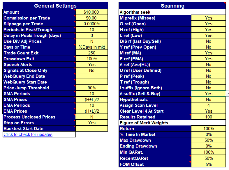
For any given trading day, we typically backtest 250 days of price data ending on the day in question using over 100 algorithms (pre-selected from about 400,000) and sort those algorithms based on performance. We now look at the top N algorithms, where N is typically 10 to 50. Since all SignalSolver backtests end up in either a buy (bullish) or a sell (bearish) state we calculate the sentiment by taking the ratio of bullish algorithms to total algorithms.

Showing the Algorithms tab with Bullish-Bearish Sentiment

Each SignalSolver algorithm has a bullish or bearish sentiment

The sentiment for any given date may vary depending on the backtester settings and other factors.

Walk forward

The simulations calculate the sentiment for a single day (or week or month) at a time and then walk forward to the next trading day. On each cycle, the backtested algorithms are sorted  by performance  and the sentiment derived as described above. The included algorithms can change from day to day due to sorting.  There may also be periodic changes to the algorithm set or their parameters in order to maintain the quality of the backtests.

As the simulation proceeds, one new OHLC data point is included and one old data point is excluded from the backtests.

Signalling thresholds

To trade using the sentiment indicator, we must somehow generate buy and sell signals and to do that we use simple threshold crossing. In the program you can define the buy and sell thresholds separately but for most of the simulations, we will set the buy threshold equal to the sell threshold, usually 50%. Crossing above 50% is a buy signal, crossing below 50% is a sell signal.

Occasionally we will show examples of simulations with a biased (non 50%) threshold. Occasionally we allow the program to optimize the thresholds periodically. We can even use inverted thresholds in which the buy will occur as the sentiment crosses below the threshold, and the sell above. When trading using SignalSolver Sentiment, its all about understanding and manipulating the thresholds.

Simulated trading using sentiment signals

Since we use Open High Low Close data and current price, we can simulate two types of trading. We can either

  1. Take a sentiment reading after the close and trade at the next open
  2. Take a sentiment reading just before the close and trade at the close

The first type of simulation will be slightly more accurate than the second, but if trading live you may have been able to fill orders at better or worse prices than the simulation indicates. Note that in type 1. simulations, the trading prices are always "out-of-sample", that is, the trading data points are outside of the backtest data. In type 2. simulations, the last price in the backtests is assumed to be the trading price, but in reality the trading price will still be out-of-band and could be slightly better or worse. But if you assume these errors are small and tend to cancel each other out, the simulations will end up being fairly accurate.
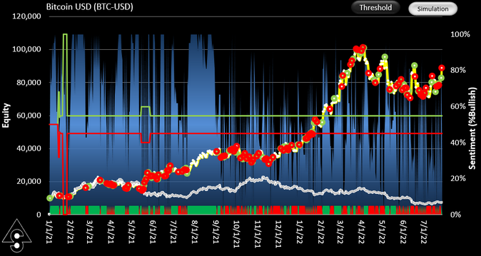
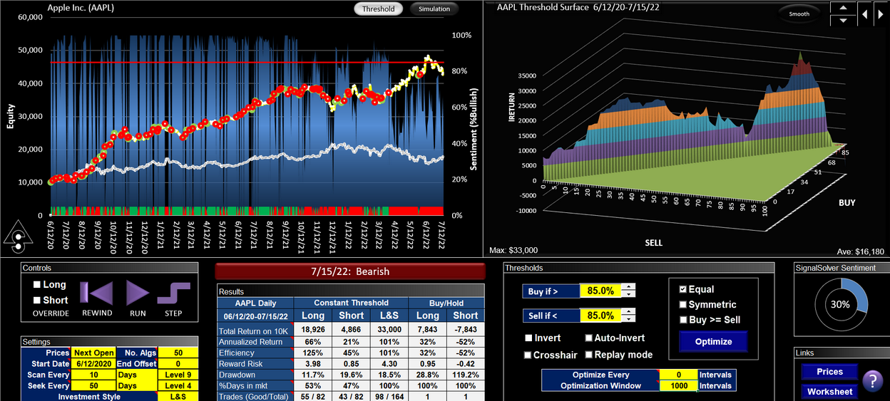
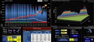
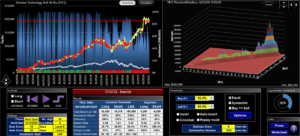
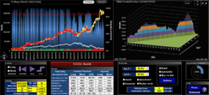
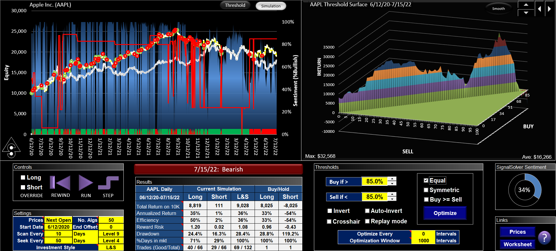
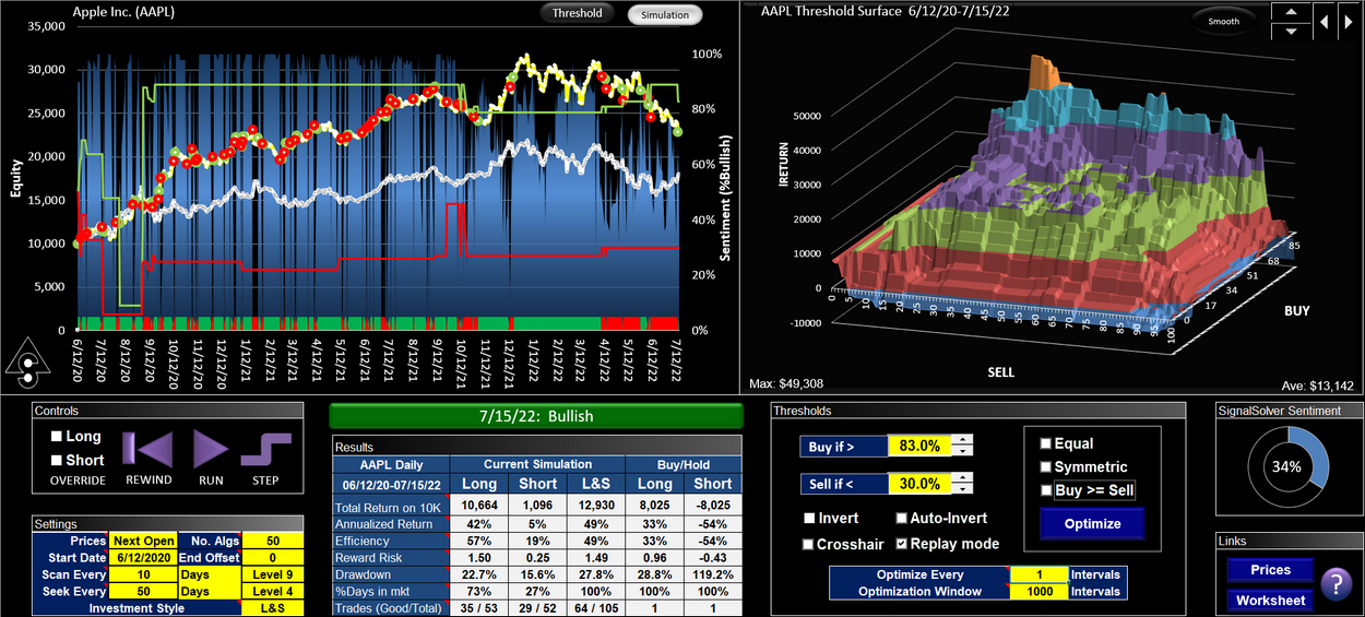
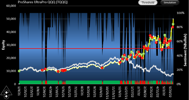
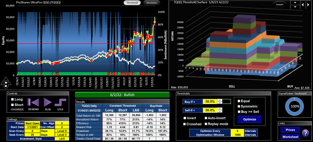
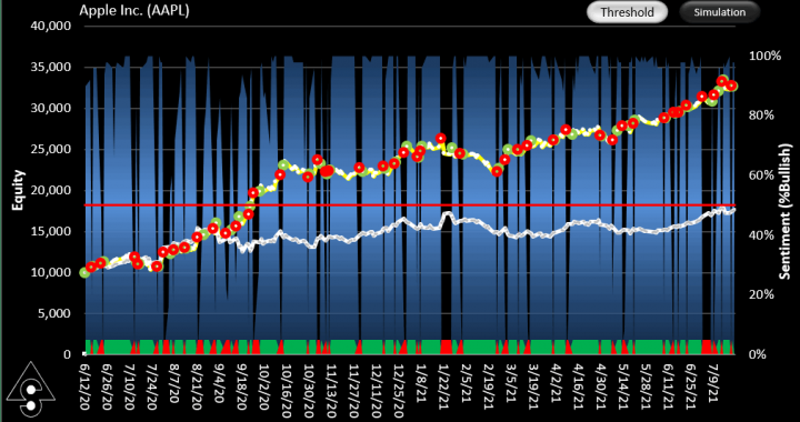
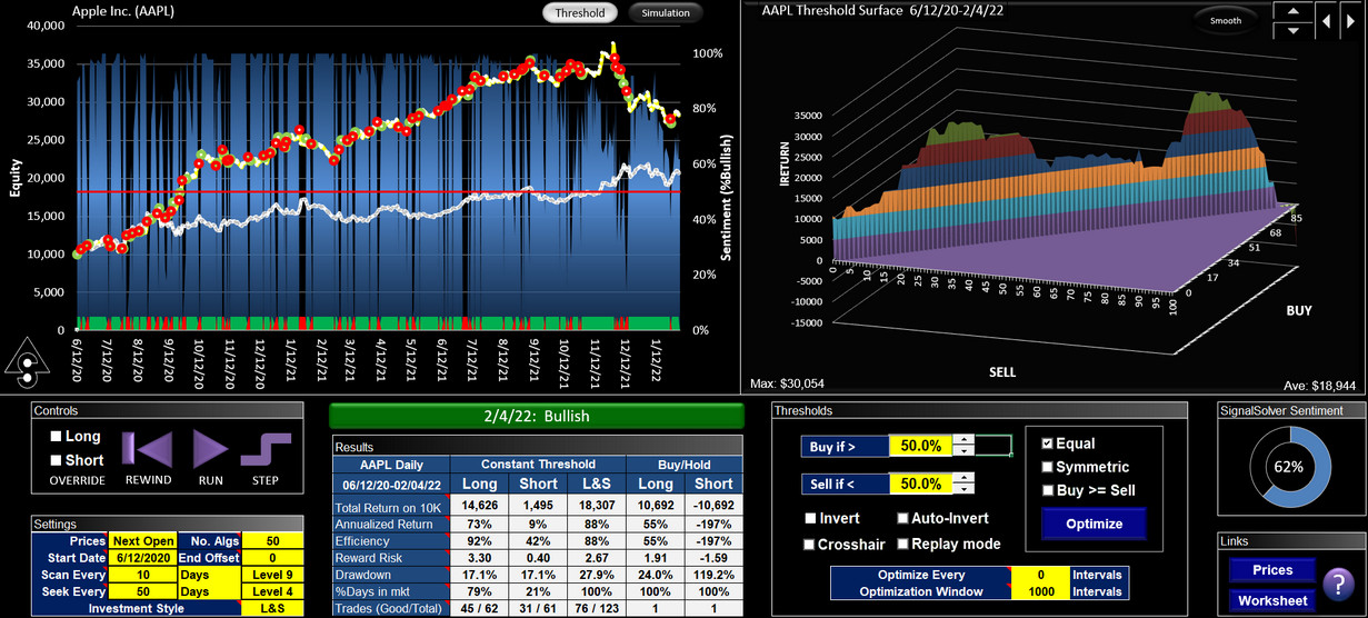
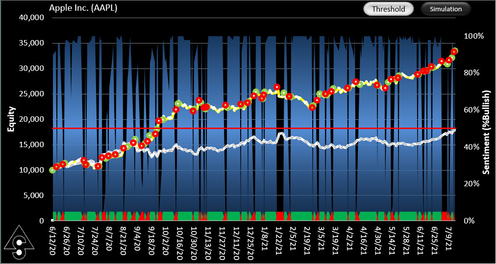
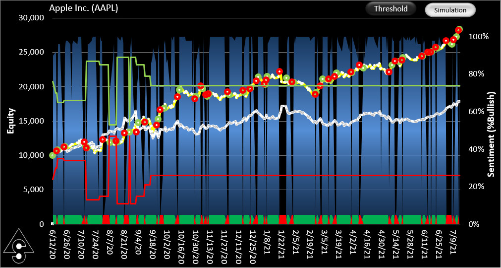
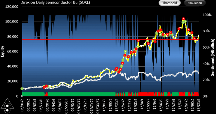
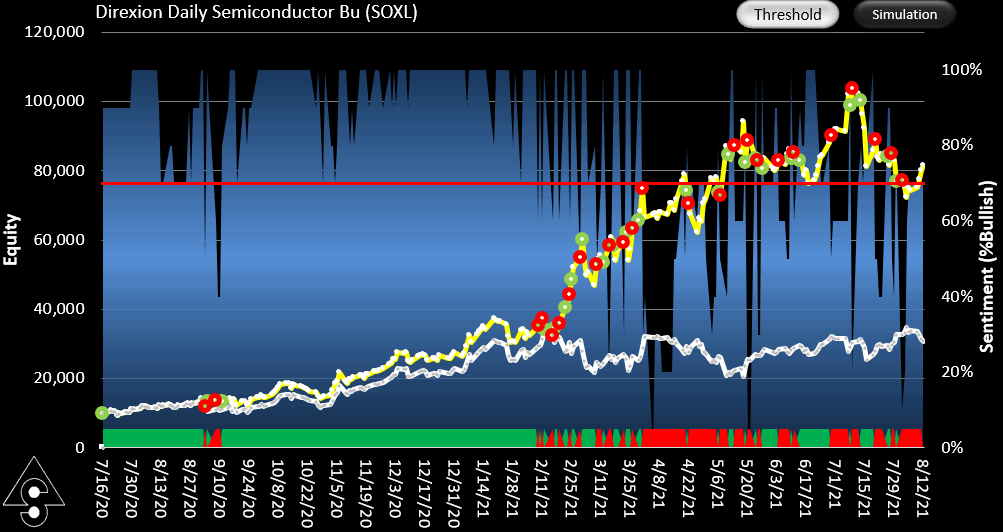
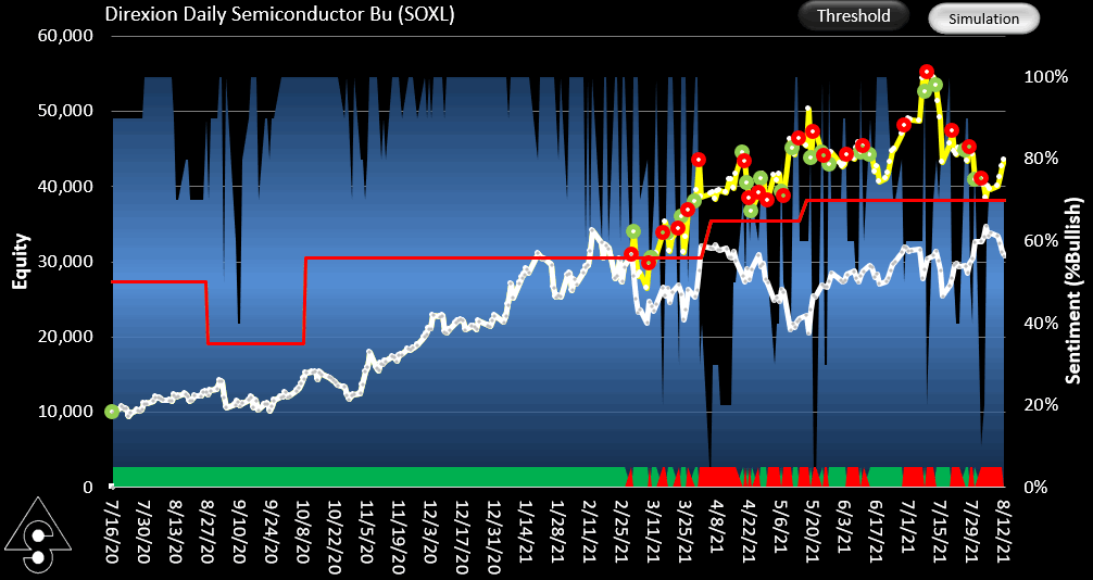
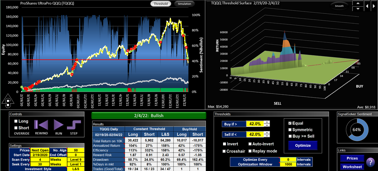
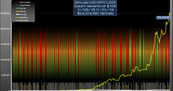
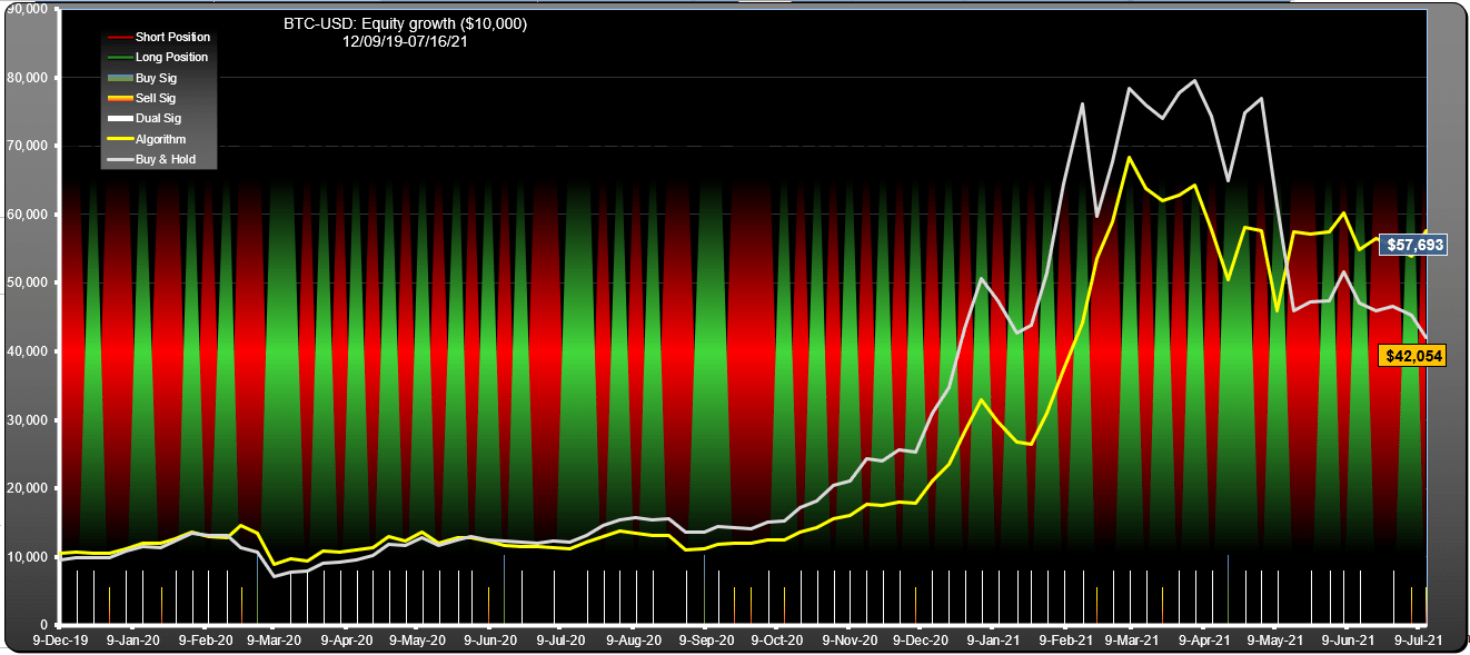
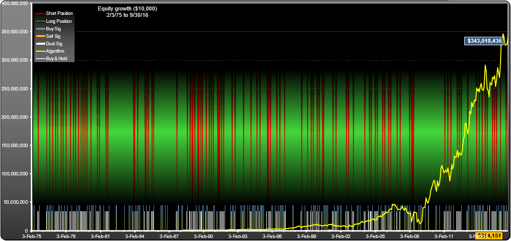
Equity Curves

There are two types of Equity Curves; Threshold view and Simulation view. They both show the result of investing $10,000.

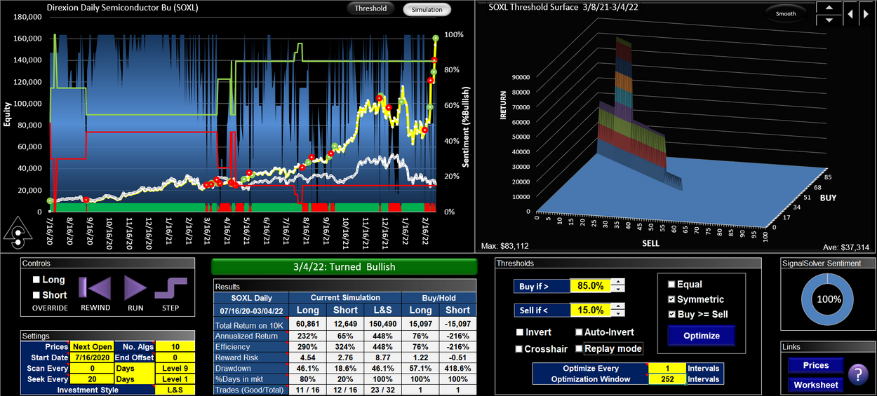
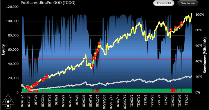
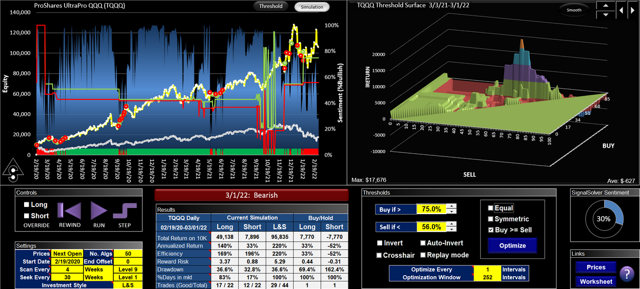
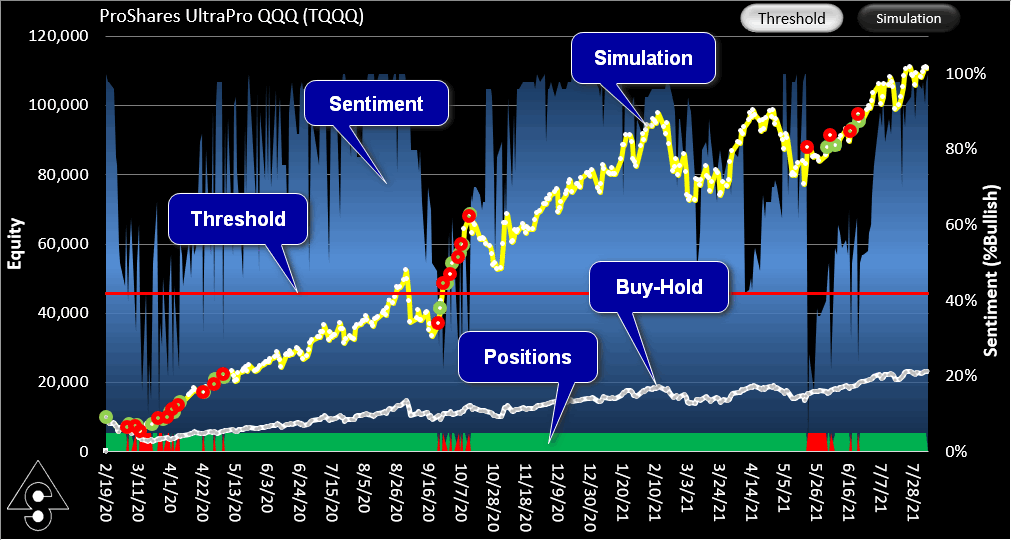
Simulation View Equity Curve

Simulation view shows the result of simulating actual trading using sentiment with no prior knowledge about thresholds. It shows what actually would have happened had you adjusted the thresholds day to day (or had the program do it for you).

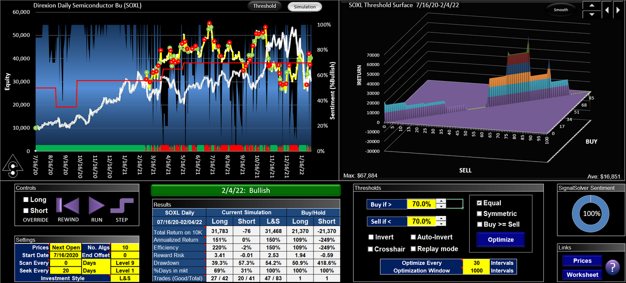
In the example below, the program automatically optimized the thresholds every 5 days, with buy and sell thresholds constrained to be equal. You can see that the thresholds converged on a value of 43%, ending up on a value of 42%.

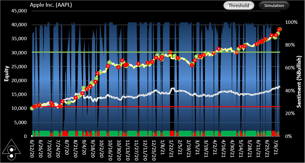
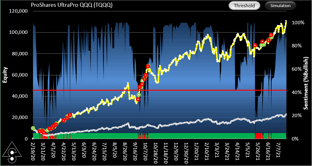
If you are curious to know what would have happened if you had started out with a 42% threshold, you can find out by looking at the Threshold view.

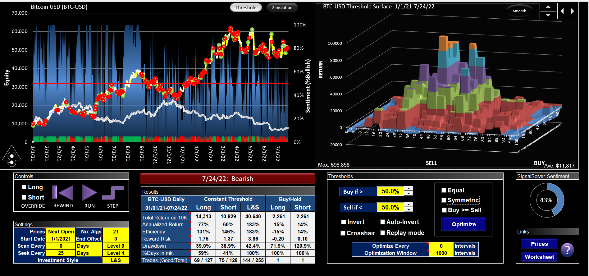
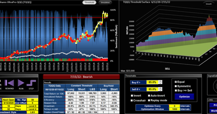
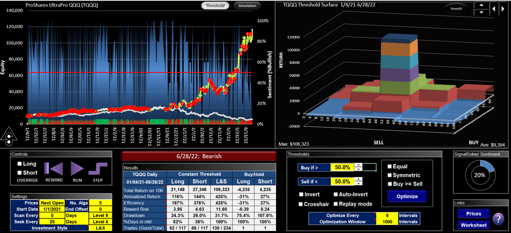
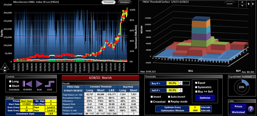
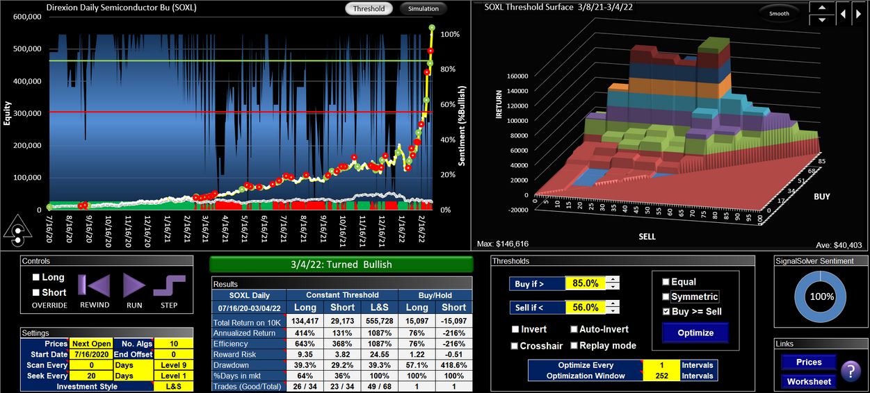
Threshold View Equity Curve

Threshold view shows the equity curve for a constant threshold. Below is the same TQQQ sentiment profile with a 42% threshold. It gives a better result but you would need a time machine to realize it. Simulation view shows what could readily have been realized if you had started cold on day one with no knowledge of threshold behavior. It's important to understand this distinction. But when you are making threshold decisions, Threshold view turns out to be very useful.
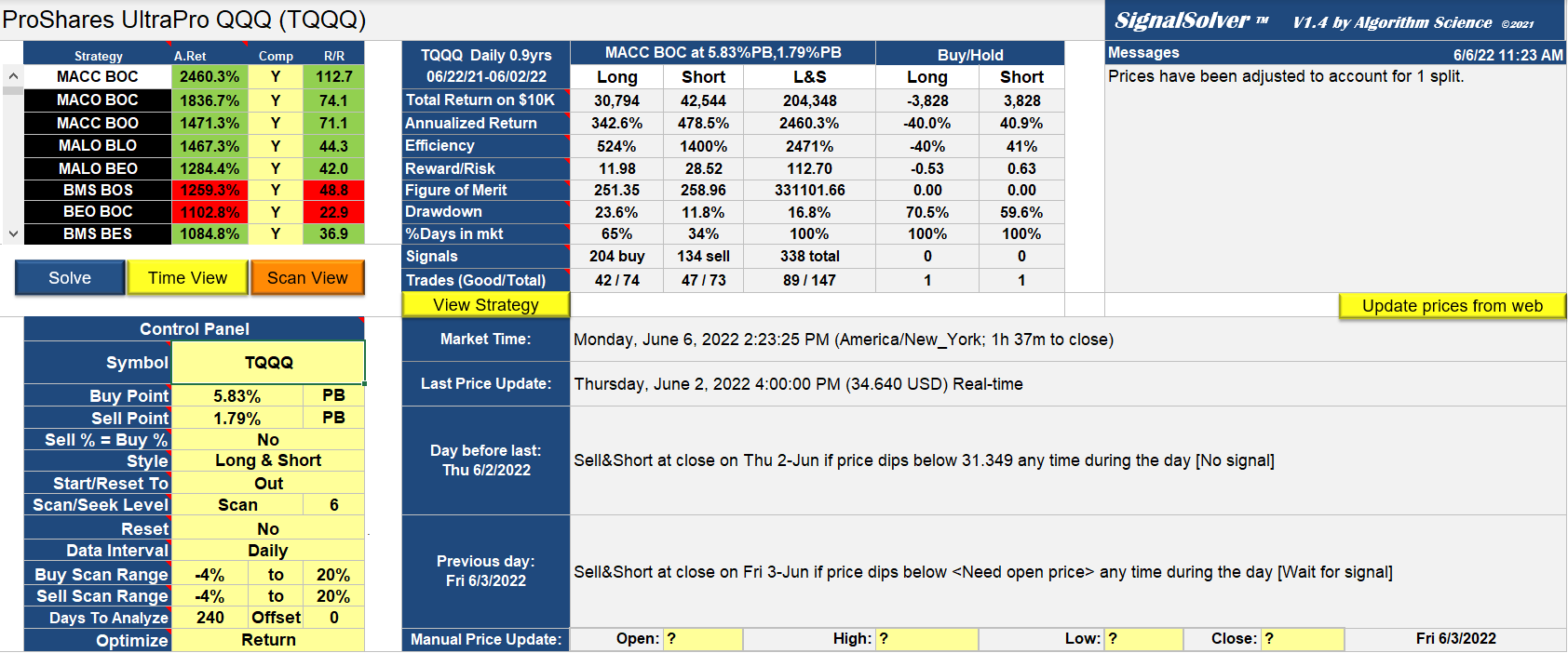
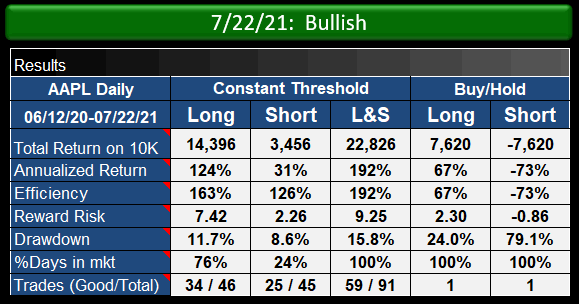
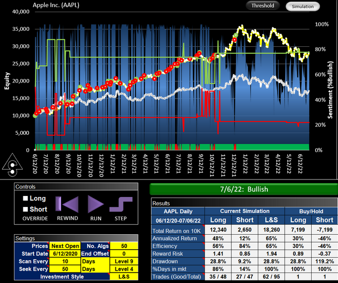
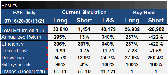
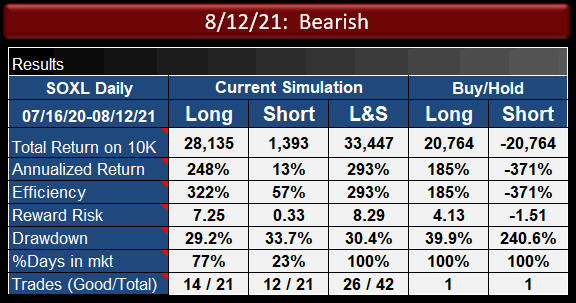
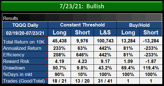
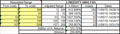
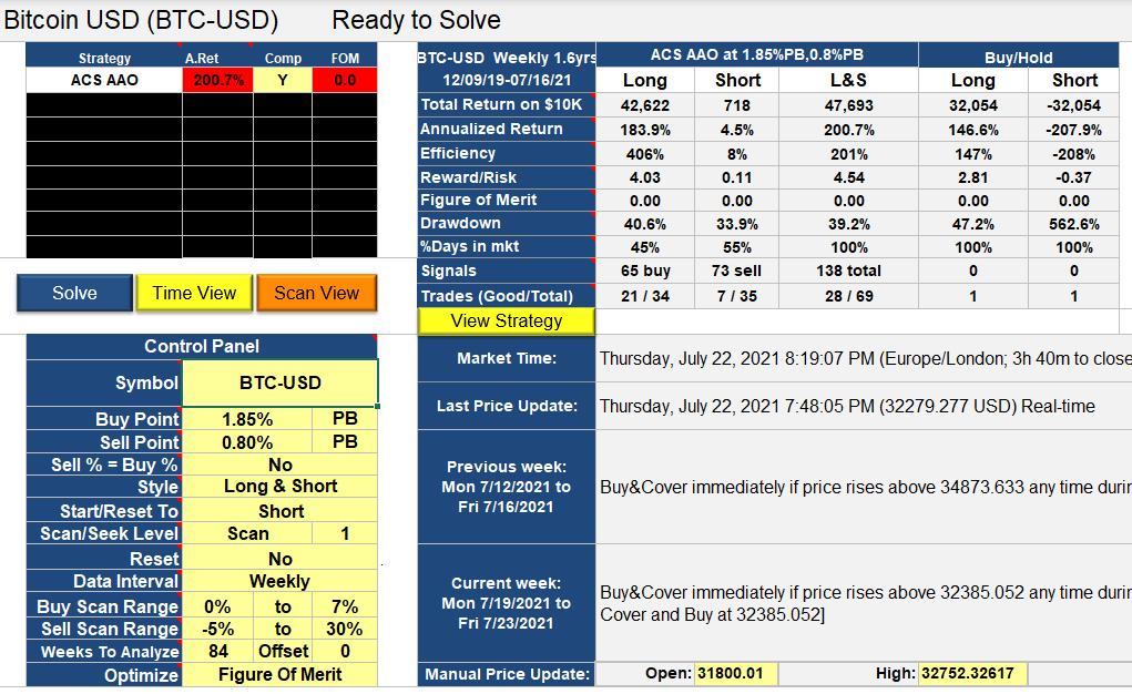
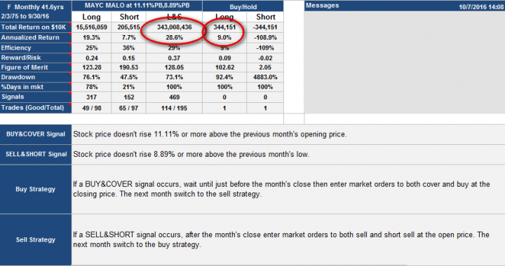
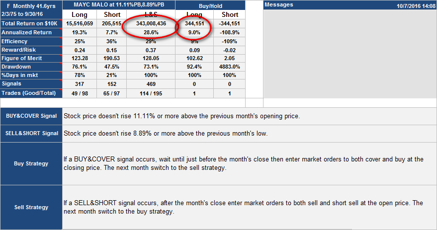
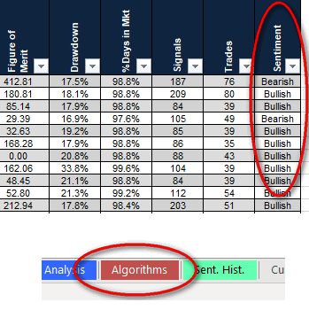
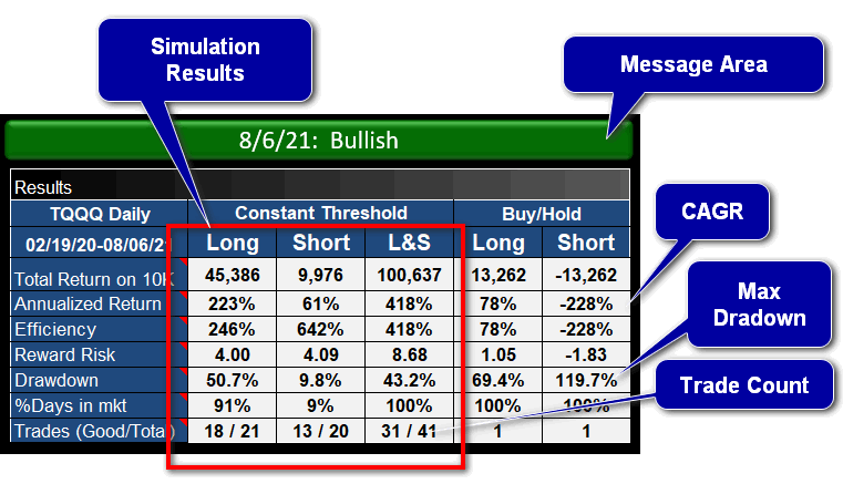
Performance tables

Below is shown the performance table for the Threshold view above. Again, these tables can be for Threshold or Simulation view, this one is for Constant Threshold. The message area informs the user what the sentiment is for the current date and if a change has occurred.

  • Annualized Return is also known as the Compounded Annual Growth Rate (CAGR).
  • Efficiency is relevant if you are out-of-the-market for some of the period. It is the Annualized Return if you had realized the return for the entire period.
  • Reward-Risk is the Annualized Return divided by (Drawdown + 5%).
  • Drawdown is the worst case loss if you had entered the strategy on a high and exited at a subsequent low.
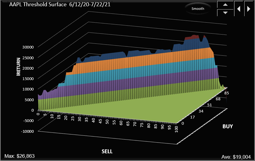
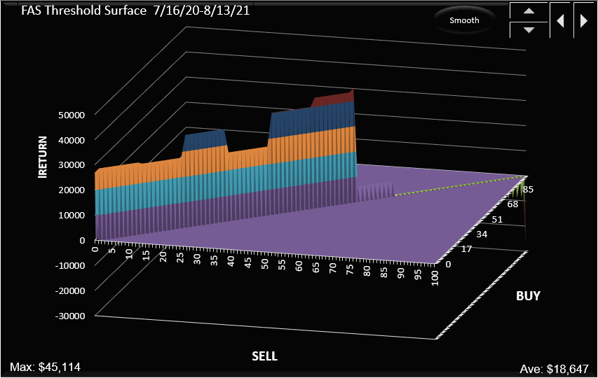
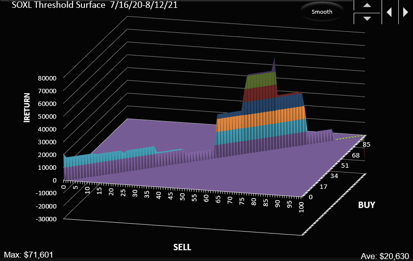
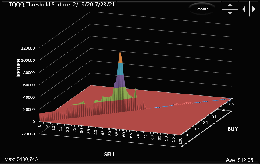
Threshold Surface

The Threshold Surface is a 3D chart showing the return for values of buy and sell threshold. Sometimes we show a partial surface, for example below we are showing only the surface for when the buy and sell thresholds are equal. You can see the peak at 42%.

We hope this explains how sentiment works and what the charts and tables in the postings represent.

You can read more about sentiment here

Bitcoin (BTC-USD) Signals-Weekly (ACS AAO)

Original Post Nov 2019:

While shorting Bitcoin might be tricky, with this algorithm it would have paid off. Traded as directed these signals would have performed around 103.1 times better than buy-hold for the period 09-Nov-15 to 01-Nov-19.

The trading signals for Bitcoin USD (BTC-USD) were selected for their reward/risk, longevity and parameter sensitivity characteristics. Backtests don't always generate reliable signals which can be counted on moving forward but many traders find value in knowing what buy and sell signals would have worked well in the past.

Bitcoin Signals (BTC-USD)

The trading signals for Bitcoin USD (BTC-USD) were selected for their reward/risk, longevity and parameter sensitivity characteristics. Backtests don't always generate reliable signals which can be counted on moving forward but many traders find value in knowing what buy and sell signals would have worked well in the past.

Returns for the Bitcoin USD (BTC-USD) signals

For the 208 week (4.0 year) period from Nov 9 2015 to Nov 1 2019, these signals for Bitcoin USD (BTC-USD) traded both long and short would have yielded $24,314,581 in profits from a $10,000 initial investment, an annualized return of 612.9%. Traded long only (no short selling) the signals would have returned $3,629,957, an annualized return of 341.8%. 42.5% of time was spent holding the currency long. The return would have been $235,929 (an annualized return of 124.1%) if you had bought and held Bitcoin for the same period. Minimum annual return for the four years in the analysis was 258.89%

Signals and Trades

We call this a weekly strategy as weekly OHLC data is used in the numerical analysis leading to at most one buy signal and one sell signal per week. However, not all signals result in trades. If you are already long in a security, buy signals are not acted upon, similarly if you are short you should ignore sell signals. There were 145 buy signals and 170 sell signals for this particular BTC-USD strategy which in turn led to 80 round trip long trades of which 56 were profitable, and 80 short trades of which 22 were profitable. There were only 15 clear buy signals and 40 clear sell signals, the remaining 130 signals were dual signals (buy and sell signals in the same week), which leads to a lot of reversals. Despite all the signal noise, drawdown was fairly constrained.

Drawdown and Reward/Risk

Drawdown (the worst case loss for an single entry and exit into the strategy) was 26% for long-short and 25% for long only. This compares to 83% for buy-hold. The reward/risk for the trading long and short was 19.70 compared to 1.41 for buy-hold, a factor of 14.0 improvement. If traded long only, the reward/risk was 11.50. We use drawdown plus 5% as our risk metric, and annualized return as the reward metric.

The backtests assume a commission per trade of $7.

Trade List

Click to see trades

Trade Types -

"Buy S" -- buy at signal price (initiated by a stop-buy order)
"RvS O" -- reversal to short at open (market sell and short orders)
"RvL S" -- reversal to long at the signal (stop-cover and stop-buy orders)

Date Trade Type Price Equity Value (at open)
10,000
11/16/2015 Buy S 326.09 9,940
11/23/2015 RvS O 371.44 11,369
11/30/2015 RvL S 378.16 11,497
12/7/2015 RvS O 433.27 12,760
12/14/2015 RvL S 441.78 12,525
12/21/2015 RvS O 423.34 11,960
12/28/2015 RvL S 430.65 11,723
1/4/2016 RvS O 448.70 12,217
1/18/2016 RvL S 389.37 14,278
2/1/2016 RvS O 376.76 13,357
2/8/2016 RvL S 383.59 13,920
2/15/2016 RvS O 438.99 14,979
3/7/2016 RvL S 415.25 15,735
3/14/2016 RvS O 413.42 15,692
3/21/2016 RvL S 421.41 15,562
3/28/2016 RvS O 421.30 15,356
4/11/2016 RvL S 429.36 14,987
4/18/2016 RvS O 459.12 16,077
4/25/2016 RvL S 467.04 15,275
5/2/2016 RvS O 458.21 15,473
5/23/2016 RvL S 447.45 18,688
5/30/2016 RvS O 574.60 20,305
6/6/2016 RvL S 585.61 22,826
6/13/2016 RvS O 763.93 25,948
6/27/2016 RvL S 641.01 30,944
7/4/2016 RvS O 648.48 30,446
7/11/2016 RvL S 661.37 30,658
7/18/2016 RvS O 661.26 29,808
8/15/2016 RvL S 581.03 33,427
8/22/2016 RvS O 574.07 32,996
8/29/2016 RvL S 584.53 33,736
9/5/2016 RvS O 607.01 33,612
9/26/2016 RvL S 611.94 33,272
10/3/2016 RvS O 616.82 33,577
10/10/2016 RvL S 628.16 33,662
10/17/2016 RvS O 657.16 34,452
10/24/2016 RvL S 669.23 35,494
10/31/2016 RvS O 710.74 35,889
11/7/2016 RvL S 724.69 34,069
11/14/2016 RvS O 731.27 35,476
11/21/2016 RvL S 744.55 34,253
11/28/2016 RvS O 773.39 36,152
12/12/2016 RvL S 783.97 35,949
12/19/2016 RvS O 896.91 40,764
12/26/2016 RvL S 912.76 43,795
1/3/2017 RvS O 913.24 40,037
1/17/2017 RvL S 837.00 47,950
1/23/2017 RvS O 920.15 47,659
1/30/2017 RvL S 936.51 51,390
2/6/2017 RvS O 998.89 49,901
2/13/2017 RvL S 1,017.67 50,441
2/21/2017 RvS O 1,163.78 55,963
2/27/2017 RvL S 1,186.76 58,574
3/6/2017 RvS O 1,221.78 56,448
3/13/2017 RvL S 1,243.98 46,201
3/20/2017 RvS O 972.05 43,283
3/27/2017 RvL S 984.61 47,844
4/3/2017 RvS O 1,187.30 51,488
4/17/2017 RvL S 1,204.82 50,917
4/24/2017 RvS O 1,348.30 56,740
5/1/2017 RvL S 1,372.83 64,785
5/8/2017 RvS O 1,808.44 73,352
5/15/2017 RvL S 1,842.37 79,805
5/22/2017 RvS O 2,159.43 84,331
5/30/2017 RvL S 2,195.68 94,860
6/5/2017 RvS O 2,953.22 111,490
6/19/2017 RvL S 2,595.43 124,749
7/3/2017 RvS O 2,525.25 121,589
7/17/2017 RvL S 1,965.52 206,498
7/24/2017 RvS O 2,763.24 208,792
7/31/2017 RvL S 2,808.19 234,972
8/7/2017 RvS O 4,066.10 297,367
8/14/2017 RvL S 4,148.62 287,236
8/21/2017 RvS O 4,384.45 307,865
8/28/2017 RvL S 4,463.96 310,912
9/5/2017 RvS O 4,122.47 279,130
9/11/2017 RvL S 4,199.21 234,251
9/18/2017 RvS O 3,681.58 240,140
9/25/2017 RvL S 3,750.97 276,102
10/2/2017 RvS O 4,614.52 289,825
10/9/2017 RvL S 4,695.77 344,841
10/16/2017 RvS O 6,006.00 364,134
10/23/2017 RvL S 6,119.58 356,958
10/30/2017 RvS O 7,403.22 432,153
11/6/2017 RvL S 7,544.45 333,649
11/13/2017 RvS O 8,039.07 451,673
11/20/2017 RvL S 8,185.17 506,705
11/27/2017 RvS O 11,315.40 613,024
12/4/2017 RvL S 11,532.68 804,284
12/11/2017 RvS O 19,106.40 996,069
12/26/2017 RvL S 14,183.43 1,246,412
1/2/2018 RvS O 16,476.20 1,455,190
1/16/2018 RvL S 14,026.78 1,386,266
1/22/2018 RvS O 11,755.50 1,400,838
2/5/2018 RvL S 8,430.13 1,735,545
2/12/2018 RvS O 10,552.60 2,249,531
2/20/2018 RvL S 10,747.01 1,986,676
2/26/2018 RvS O 11,532.40 2,369,426
3/12/2018 RvL S 9,755.83 2,338,739
3/19/2018 RvS O 8,498.47 2,381,987
4/2/2018 RvL S 6,970.85 2,839,760
4/9/2018 RvS O 8,337.57 3,361,090
4/16/2018 RvL S 8,483.20 3,423,511
4/23/2018 RvS O 9,426.11 3,669,416
4/30/2018 RvL S 9,593.33 3,623,968
5/7/2018 RvS O 8,713.10 3,273,579
5/29/2018 RvL S 7,504.53 3,835,916
6/4/2018 RvS O 6,799.29 3,377,313
6/18/2018 RvL S 6,619.51 3,232,228
6/25/2018 RvS O 6,380.38 3,341,357
7/2/2018 RvL S 6,503.96 3,413,215
7/9/2018 RvS O 6,357.01 3,202,581
7/16/2018 RvL S 6,477.29 3,596,687
7/23/2018 RvS O 8,221.58 3,988,065
8/13/2018 RvL S 6,439.66 4,898,264
8/20/2018 RvS O 6,710.80 5,056,708
8/27/2018 RvL S 6,831.34 5,291,294
9/4/2018 RvS O 6,301.57 4,580,742
9/10/2018 RvL S 6,417.43 4,564,219
9/17/2018 RvS O 6,704.77 4,697,830
10/15/2018 RvL S 6,407.31 4,966,527
11/5/2018 RvS O 6,411.76 4,909,627
11/26/2018 RvL S 4,084.15 6,795,416
12/3/2018 RvS O 3,612.05 5,918,347
12/17/2018 RvL S 3,313.02 7,737,752
12/24/2018 RvS O 3,866.84 7,479,526
12/31/2018 RvL S 3,937.47 7,606,043
1/7/2019 RvS O 3,557.31 6,633,920
1/14/2019 RvL S 3,618.68 6,486,468
2/4/2019 RvS O 3,695.61 6,658,040
2/19/2019 RvL S 3,741.80 6,689,376
3/4/2019 RvS O 3,953.74 6,947,199
3/11/2019 RvL S 4,024.70 6,831,415
3/18/2019 RvS O 4,024.11 6,821,475
3/25/2019 RvL S 4,096.58 6,712,984
4/1/2019 RvS O 5,199.84 8,502,625
4/8/2019 RvL S 5,295.08 8,145,490
4/15/2019 RvS O 5,312.49 8,374,318
4/22/2019 RvL S 5,412.85 8,021,833
4/29/2019 RvS O 5,791.69 8,791,138
5/6/2019 RvL S 5,902.93 10,182,649
5/13/2019 RvS O 8,196.92 11,973,055
5/20/2019 RvL S 8,349.35 12,207,401
5/28/2019 RvS O 8,741.75 12,302,629
6/10/2019 RvL S 7,830.31 15,595,486
6/17/2019 RvS O 10,853.74 18,830,874
6/24/2019 RvL S 11,056.20 18,046,272
7/8/2019 RvS O 10,257.84 17,145,206
7/15/2019 RvL S 10,445.80 17,074,584
7/22/2019 RvS O 9,548.18 15,384,715
7/29/2019 RvL S 9,729.59 17,002,139
8/5/2019 RvS O 11,528.19 17,882,352
8/19/2019 RvL S 10,537.21 18,662,251
8/26/2019 RvS O 9,757.47 17,982,509
9/3/2019 RvL S 9,938.49 18,545,200
9/9/2019 RvS O 10,347.22 18,374,698
9/30/2019 RvL S 8,254.11 21,382,412
10/7/2019 RvS O 8,320.83 22,270,204
10/21/2019 RvL S 8,374.19 25,274,184
10/28/2019 RvS O 9,205.73 24,324,581
11/4/2019 Last 9,205.73 24,324,581

Updates

Dec 02 2019

No signal last week (7857.354). The sell signal (above 7284.448) arrived at this weeks open, but this algorithm sells at the next open, so the sell time is next week's open 12:00am GMT on Dec 9th 2019.


Update 1/9/20

Doing a bit better than the last update on 12/13/19.


Date Transaction Buy/Cover Sell/Short  Asset Value
 $           10,000
23-Oct-2019 Buy 8374.000  $           10,000
4-Nov-2019 Sell 9235.607  $           11,029
4-Nov-2019 Short 9235.607  $           11,029
4-Nov-2019 Cover 9406.209  $           10,825
4-Nov-2019 Buy 9406.209  $           10,825
9-Dec-2019 Sell 7561.795  $             8,703
9-Dec-2019 Short 7561.795  $             8,703
19-Dec-2019 Cover 7284.619  $             9,022
19-Dec-2019 Buy 7284.619  $             9,022
30-Dec-2019 Sell 7420.273  $             9,190
30-Dec-2019 Short 7420.273  $             9,190
6-Jan-2020 Cover 7548.427  $             9,031
6-Jan-2020 Buy 7548.427  $             9,031
9-Jan-2020 Last 7885.000  $             9,433

Update June 22 2021

Bitcoin algorithm performance

Since Dec 2019 to July 2021, this algorithm has performed better than bitcoin with higher gain, lower drawdown and significantly better reward-risk.

Bitcoin algorithm performs better than underlying security

Ford (F) Monthly Trading Strategy

Update May 12 2021

Thought I'd look at how this algorithm has done since publication in 2016. Annualized return was 12.4% compared with buy-hold annualized return of 3.9%.

You would probably have re-parameterized or seeked for a new algorithm over that timeframe, but its nice to know the original did OK.

Update 8/13/2017

This algorithm continues to perform well, outperforming buy-hold by 30.4% annualized over the last 10 months:

Ford Motor Company MAYC MALO algorithm update

Ford monthly MAYC MALO update Aug 2017

Notice this had a very low drawdown (1.2%).

This strategy has given about 1000x better return than buy-hold over the last 41.6 years.

f-m-tablef-m-equity