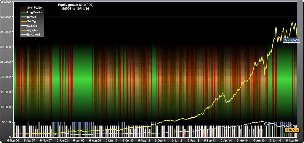
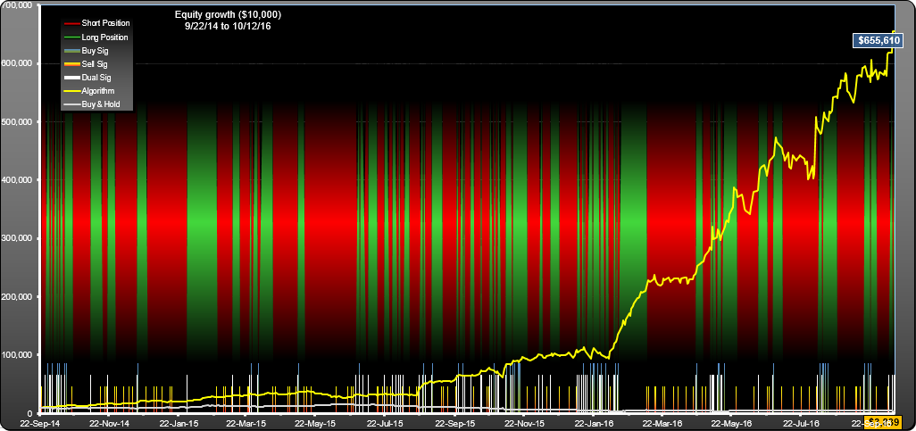
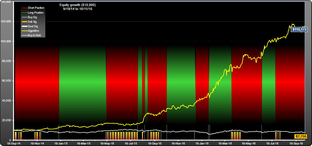
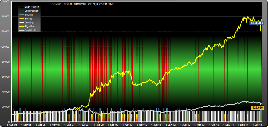
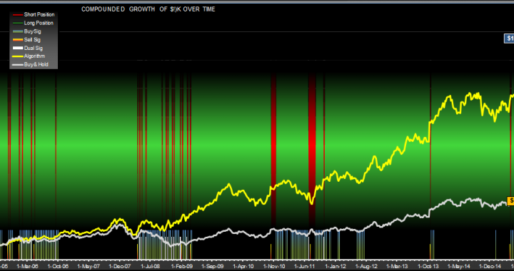
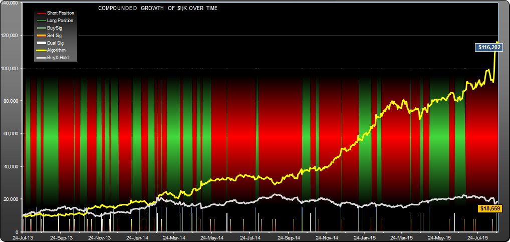
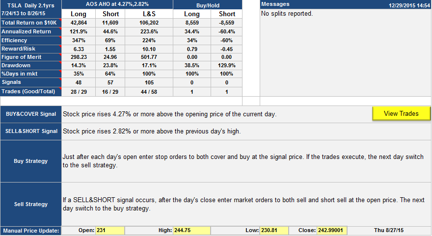
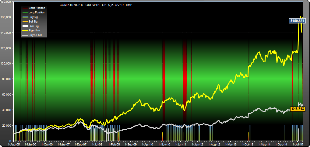
Here is a Google Inc (GOOGL) trading strategy with once a week intervention which would have performed significantly better than buy-hold over the last 10 years. Annualized return was 31.5% vs. 16.5% (returning $149K for 10K outlay vs $36.7K, compounded), drawdown was 40.2% vs. 62.4%, so reward/risk was better.
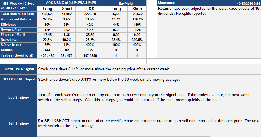
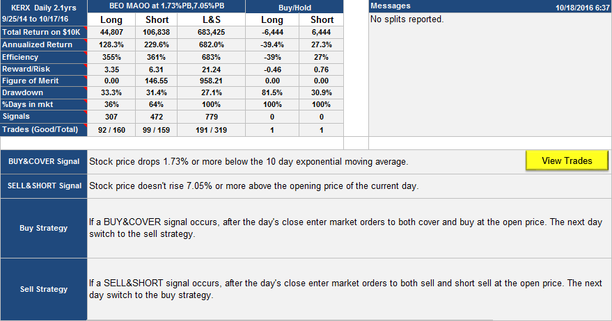
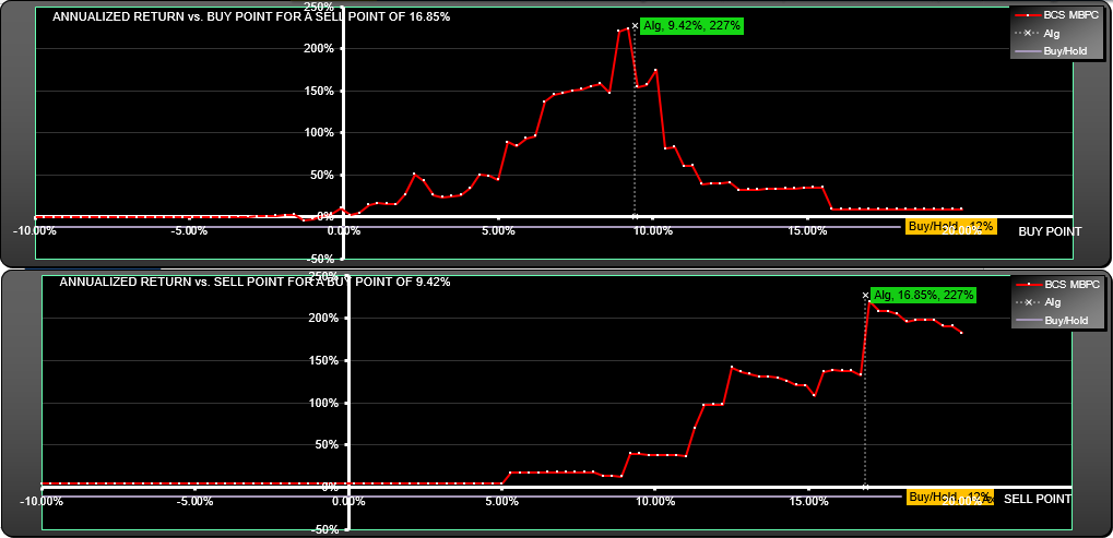
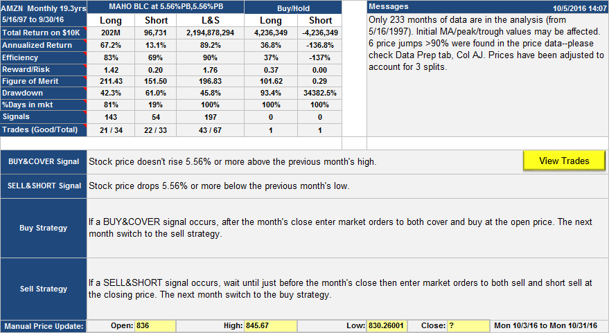
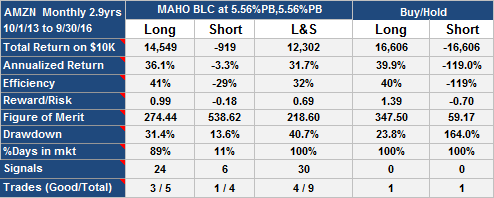
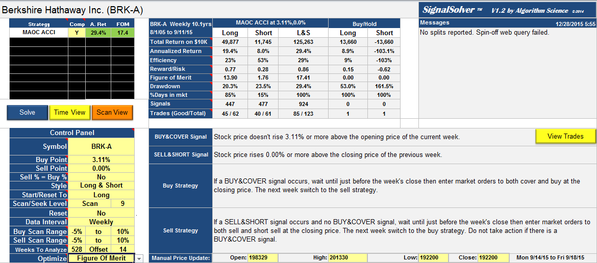
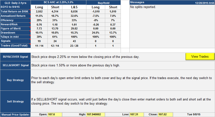
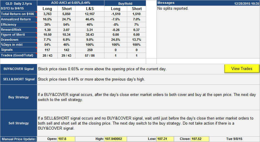
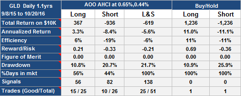
The buy and cover signal (see table below) was present every week where the price dropped 0.03% below the last price the stock was sold at which happened 174 times over the course of the 528 weeks of the analysis, and usually happened the week following a sell/short.
The sell and short signal happened every week the stock price rose 8.13% or more above the open price of the current week. This happened only 29 times, so there is a strong buy-side bias to this strategy. All trading would have been done at the open of the week following the signal.
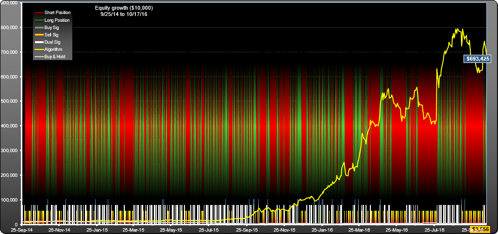
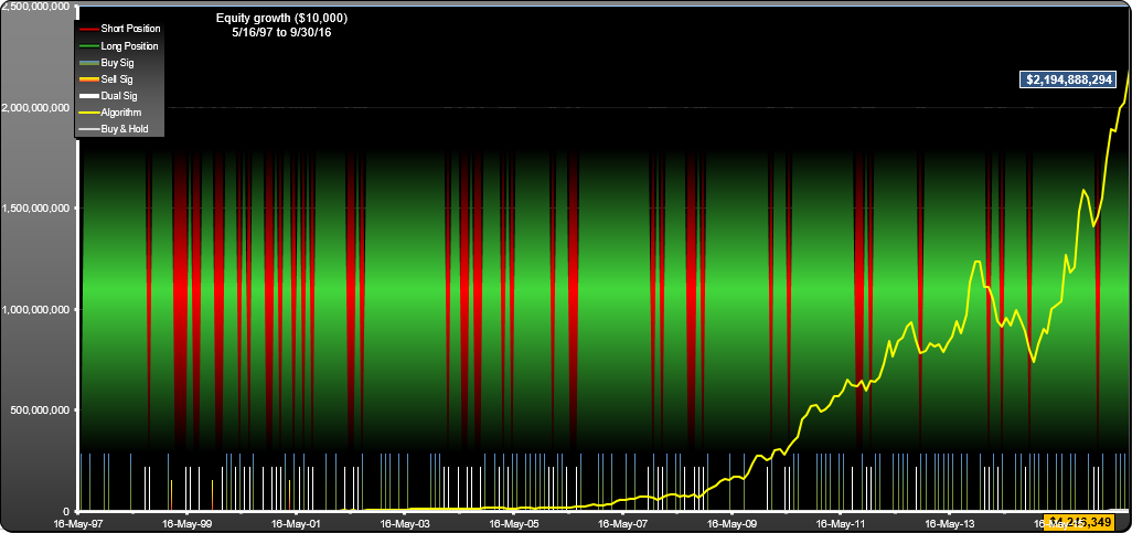
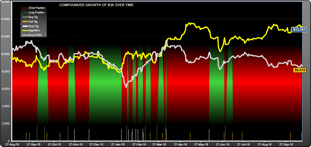
The equity curve for this GOOGL trading strategy shows that the stock was held short (the red bands in the background) for small periods, typically a week.
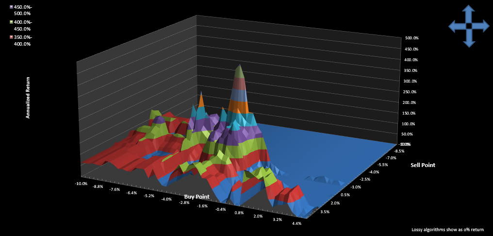
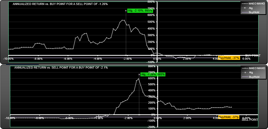
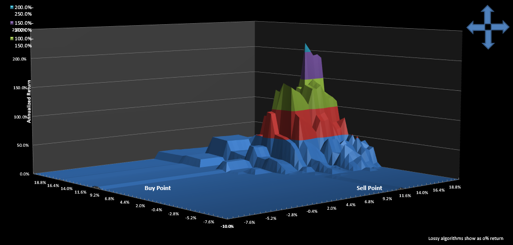
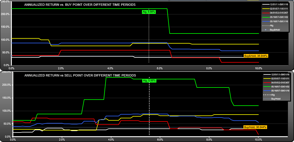
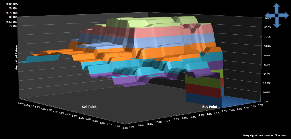
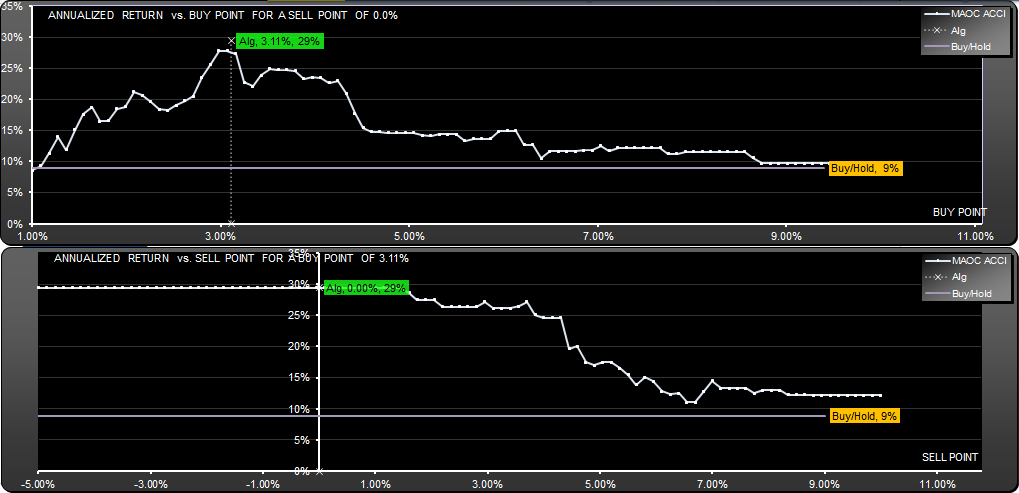
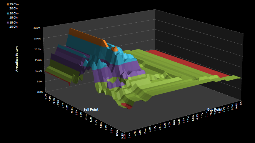
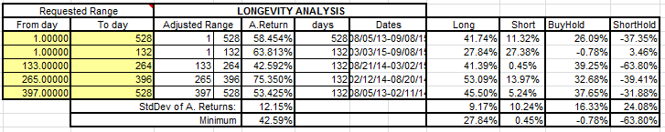
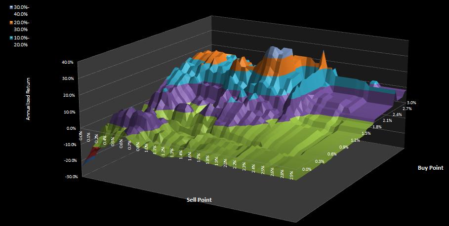
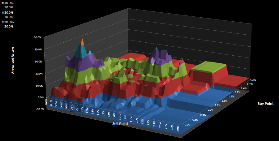
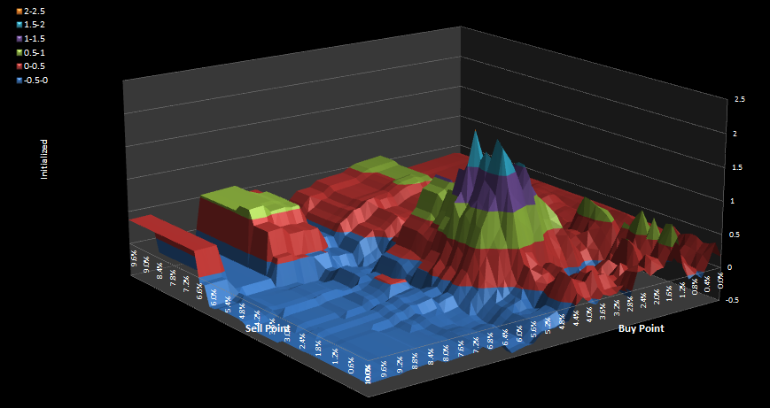
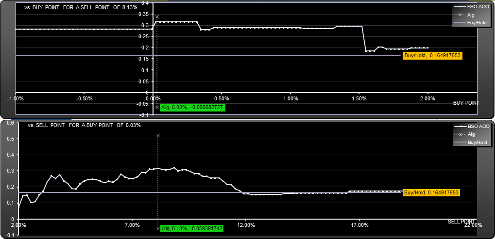
The scan below shows how the annualized return changed, had the buy and sell parameters changed. At 2.35% buy point, the algorithm gets stuck, resulting in a loss. This is characteristic of trading strategies which reference buy or sell prices. At 1.5% sell point and below, the algorithm made a loss, but returns for all buy points above that were positive, for the 0.03% buy point.
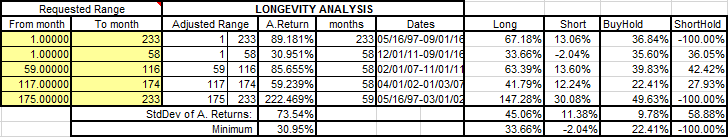
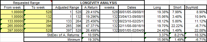
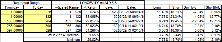
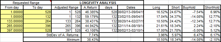
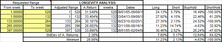
One nice characteristic this algorithm had was consistent returns for each of the 132 week periods in the backtest. You can see from the table below that the annualized return was between 28% and 34.8% for every period. Compare that with buy-hold which ranged from -4.6% to 26%
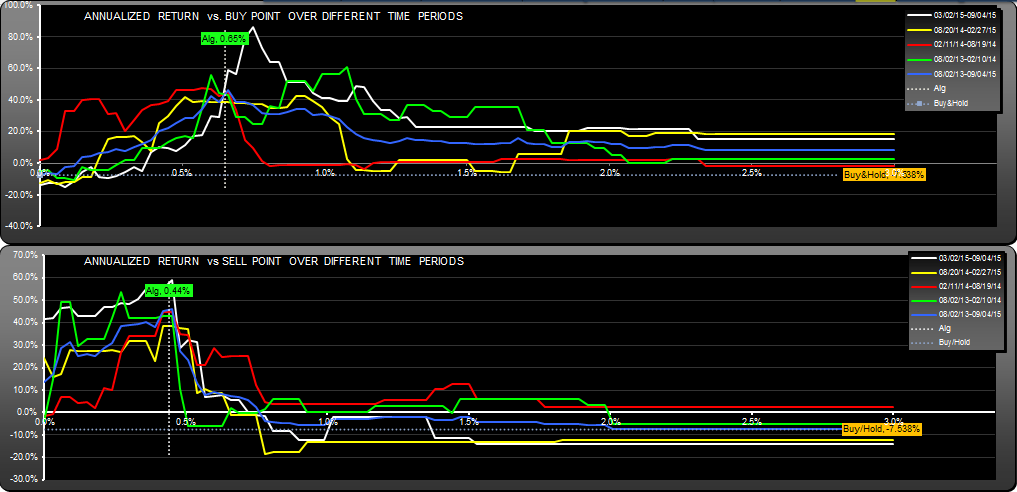
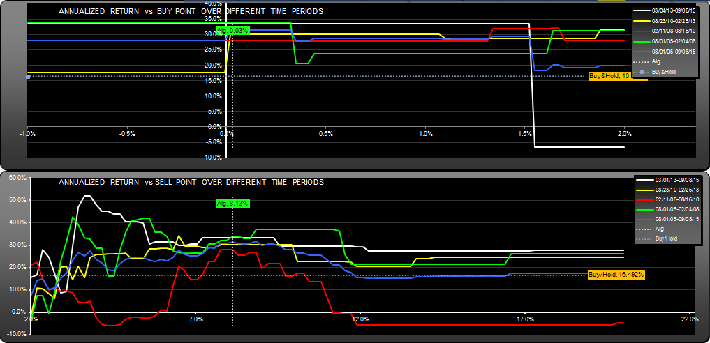
You can also see this characteristic on the scans for each quartus:
You can download the list of trades in .xlsx format: GOOGL.W Trades.
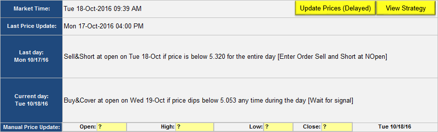
As of Sept 16th 2015, the algorithm is long, awaiting a sell signal if the price hits 708.933. Last sell price was 654.34.
Please note, while this is an interesting backtest result, it is not a suggestion to trade this way. As always I don’t know how this strategy will fare in the future, but will track it from time to time.
Andrew
This post was edited 12/28/15 to correct an error in the short-side returns.
Update Oct 21st 2016
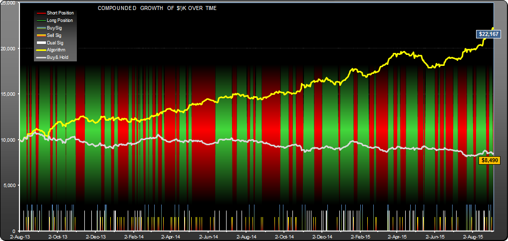
This strategy has pretty much followed buy-hold long:

GOOGL Trading Strategy Update Oct 21 2016