Original Post July 27 2021
Sentiment
Sentiment usually refers to an analyst opinion on whether a financial instrument will increase in value (bullish sentiment), or decrease (bearish sentiment). However, in this FNGU trading strategy using SignalSolver sentiment we are combining the opinion of multiple backtest algorithms to derive sentiment.
Methodology
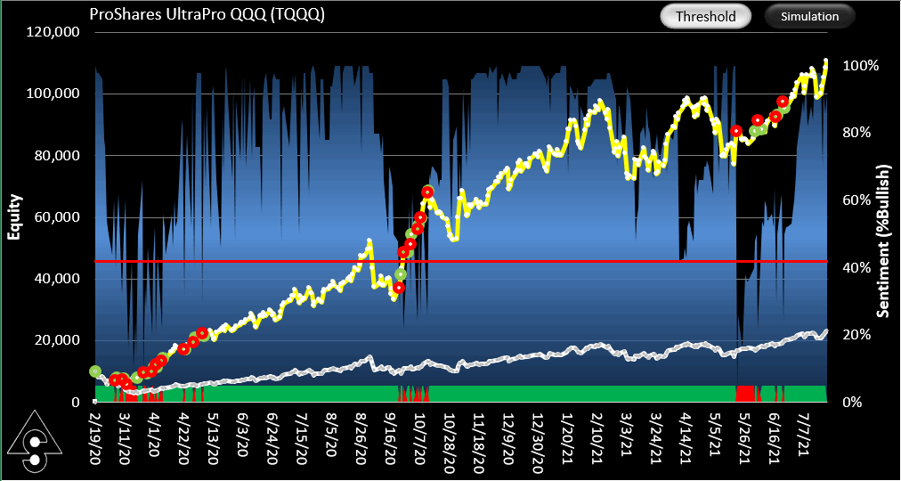
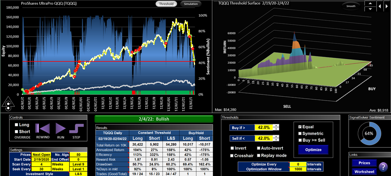
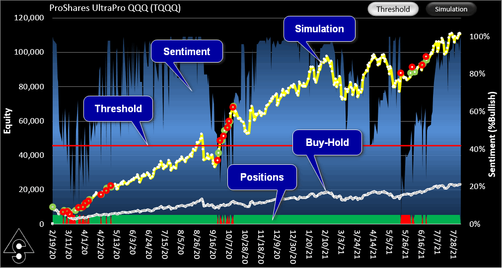
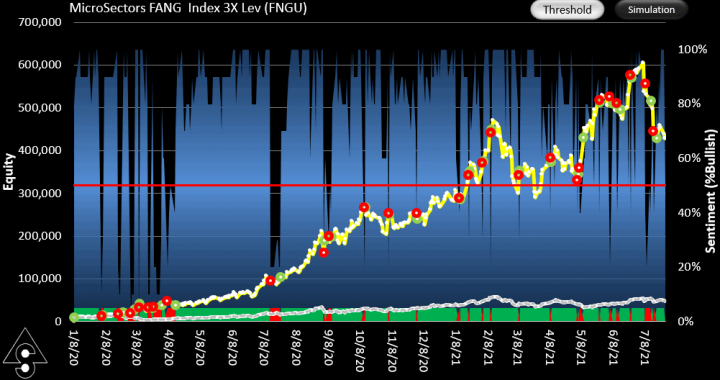
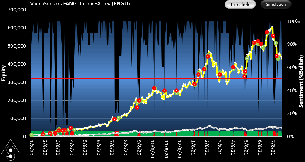
Shown above is the simulated result of trading FNGU using SignalSolver Sentiment. The sentiment is the blue area chart in the background. The equity curve for the strategy is shown in yellow, buy-hold equity in white. Sentiment is calculated each day after the close of business by assessing what percentage of the top 10 SignalSolver backtest algorithms are bullish. The top 10 are selected by sorting the 139 algorithms each day according to performance. The buy and sell thresholds are fixed at 50% (red line) with bullish being above the threshold. A trade is executed at the next open whenever sentiment crosses this threshold, so the trade price is always out-of-sample from the backtest period which is fixed at 250 trading days. The simulation then walks forward to the next day, repetitively. Algorithms are flushed and refreshed every 3 months and re-parameterized at the end of each month
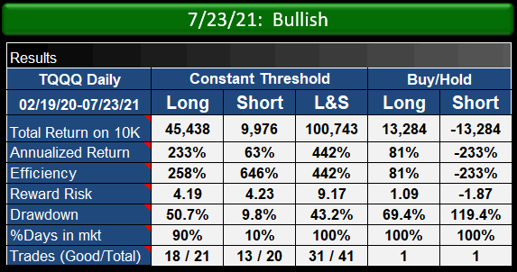
Performance
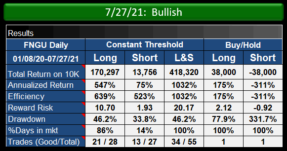
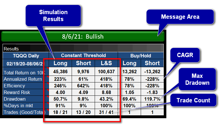
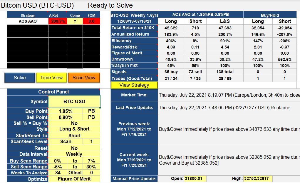
Trading on sentiment (L&S column above) performed around nine times better in this simulation than buy-hold in terms of reward/risk, with annualized return (CAGR) being around 6 times better for Long/Short trading of the signals and trading long only being about 5 times as good. In all cases, drawdown was lower for the sentiment trading than for buy-hold.
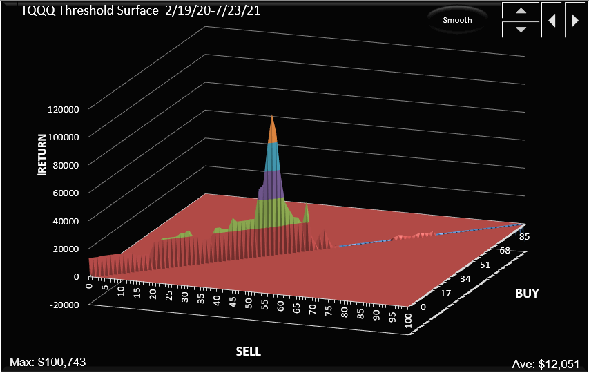
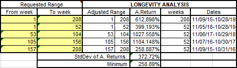
Below is shown the threshold surface for the equal buy/sell thresholds showing that annualized return (CAGR) is sensitive to threshold changes but profitable over a wide range. 50% is close to the optimum, which is at 41% through 49% ($580,959 return).
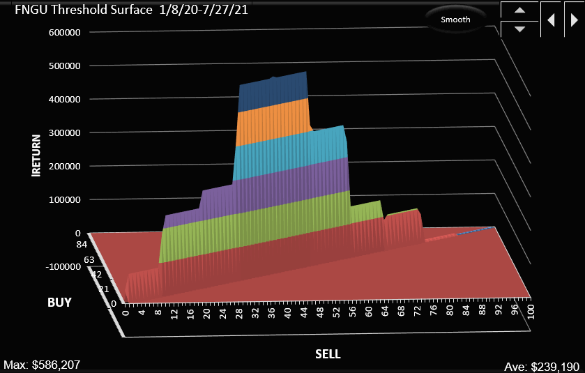
FNGU threshold surface for equal thresholds
Click here to see the SignalSolver settings for this strategy: FNGU Sentiment Settings
We now move into the paper-trading phase for this project. Updates will be shown below.
Updates
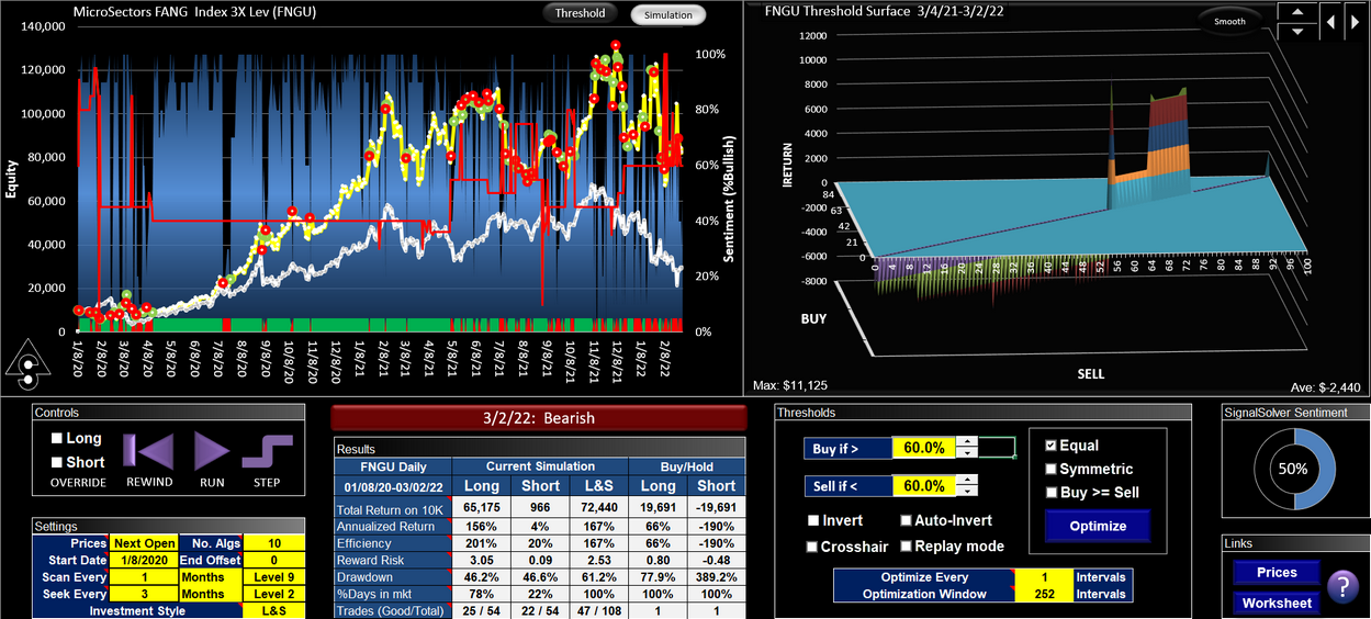
Daily updates to this strategy and sentiment were reported here, up until Feb 4th 2022 when losses on FNGU were about 19%. The screenshot below shows the progress of this algorithm. The underlying stock lost 23% in the same period.

FNGU trading using SignalSolver Sentiment. From Jan 8th 2020 until July 16th 2021 this was a backtest. From July 16th 2021 until Feb 4th 2022 it was live traded, losing 19%.
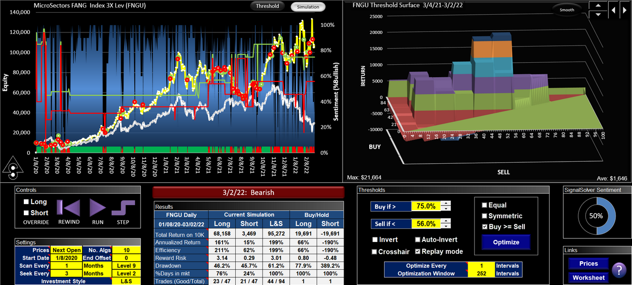
Postmortem March 3rd 2022
As we did for AAPL and TQQQ we take a look to see if something could have been done better. We start by using the same Sentiment profile and looking to see if changing the buy and sell thresholds would have made a difference. For FNGU we used a fixed 50-50 threshold because it had done such a great job in the timeframe 1/8/20 to 7/16/21. Turns out, the best Equal threshold overall (i.e. from 1/8/20) would have been 60%, but that was not guessable, not manifesting until Dec 2021. Trading from 1/8/20 with a 60% threshold would have yielded just over $900,000 in Dec 2022, falling back to $576,000 on Feb 4th 2022. For our live trading period, it would have yielded just 56%. The best Equal threshold for our trading period July 16th 2021 to Jan 4th 2022 was also 60%.
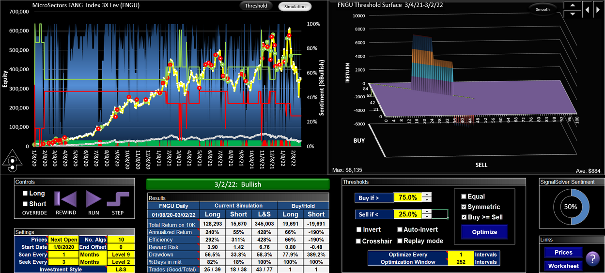
The best Symmetrical thresholds were 75% buy and 25% sell, yielding 100% profit in our trading period. Another academic result, neither guessable nor manifesting themselves until very recently.
Adaptive threshold results
We found with both AAPL and TQQQ that adaptive thresholds can give better results than fixed thresholds, so let's explore that technique a little for FNGU. With this method there is less guesswork--the program optimizes the thresholds every N periods, but you must also select how much sentiment data is in the Optimization Window. For simplicity sake we optimize every 1 period (every trading day) and we use a 252 trading day window (one calendar year). You can also force the thresholds to be Equal, Symmetrical, or allow them to float freely. Each did much better than buy-hold for the trading period which gave a 24% loss. Let's take a look at each
Equal Adaptive Thresholds
For this test the buy and sell thresholds are constrained to be equal. Overall it did better than buy-hold, but for the actual trading period (July 16th to Jan 4th '22) it gave a loss of 4%, recovering to flat since then.
Symmetrical Adaptive Thresholds
Here, we apply two constraints to the thresholds. Firstly they must sum to 100% and secondly the buy threshold must be greater or equal to the sell threshold. For the overall test period this gave the best result, and for the trading period 7/16/21 through to 2/4/22 this gave a 13.9% profit, but this has declined to a 3% loss on 3/2/22.
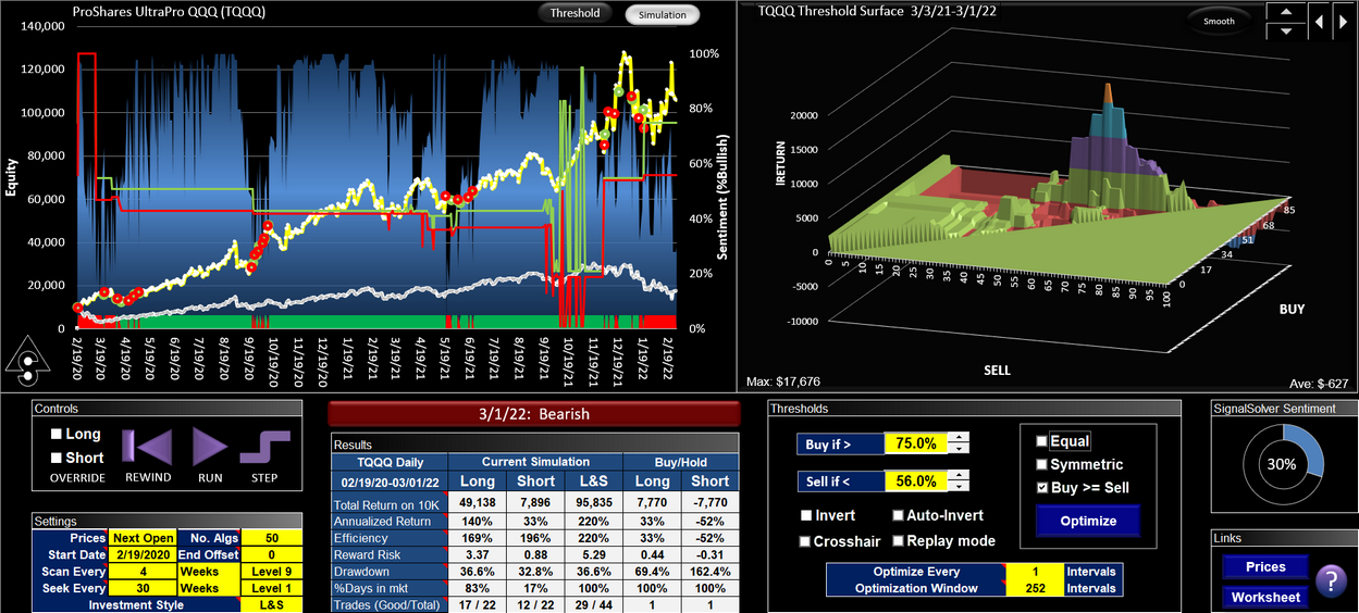
Free floating adaptive thresholds
The thresholds are re-optimized every day with the only constraint being that the buy threshold must be greater or equal to the sell threshold. This avoids the scenario where a descending sentiment causes a sell, then re-ascends without a buy (relaxing this constraint was still profitable). The result is better for the trading period 7/16/21 to 2/4/22 than either the equal or symmetrical thresholds, giving a return of 57%.. As of 3/2/22 the gain was 65% vs a 36% loss for buy-hold.