Ford (F) Monthly Trading Strategy

Update May 12 2021

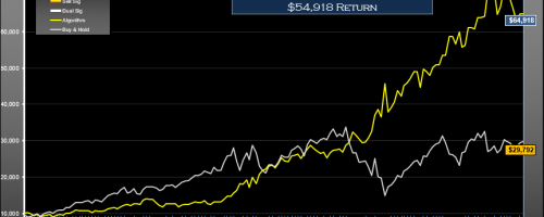
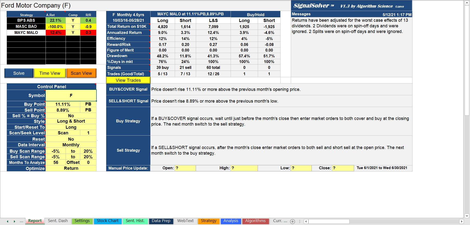
Thought I'd look at how this algorithm has done since publication in 2016. Annualized return was 12.4% compared with buy-hold annualized return of 3.9%.

You would probably have re-parameterized or seeked for a new algorithm over that timeframe, but its nice to know the original did OK.

Update 8/13/2017

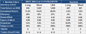
This algorithm continues to perform well, outperforming buy-hold by 30.4% annualized over the last 10 months:

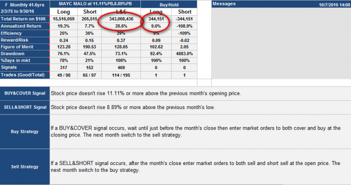
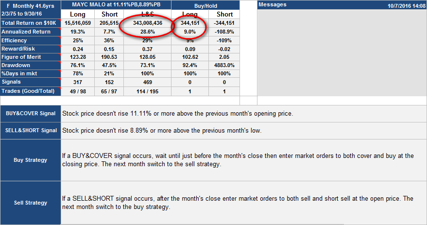
Ford Motor Company MAYC MALO algorithm update

Ford monthly MAYC MALO update Aug 2017

Notice this had a very low drawdown (1.2%).

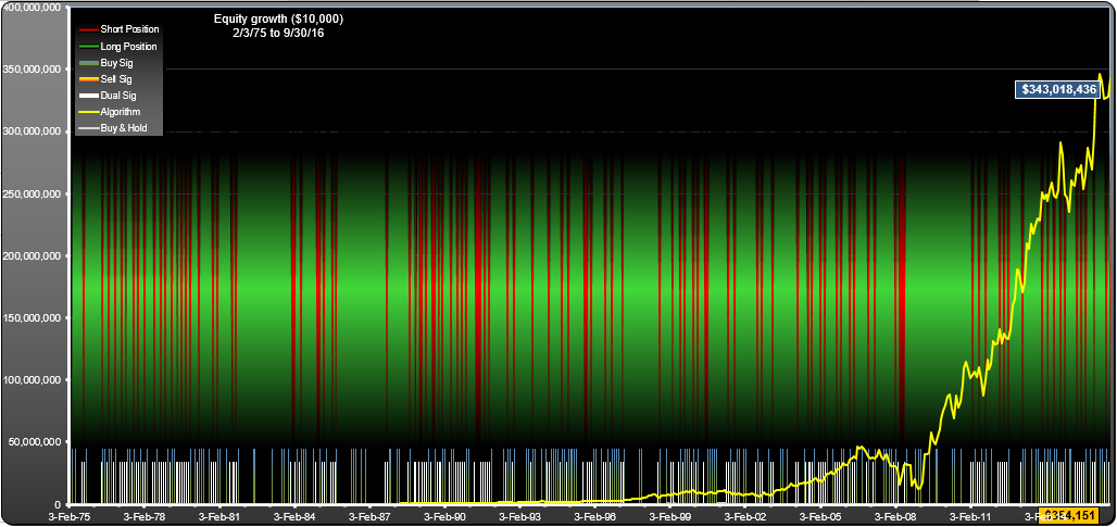
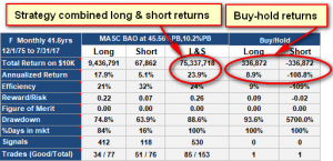
This strategy has given about 1000x better return than buy-hold over the last 41.6 years.

f-m-tablef-m-equity

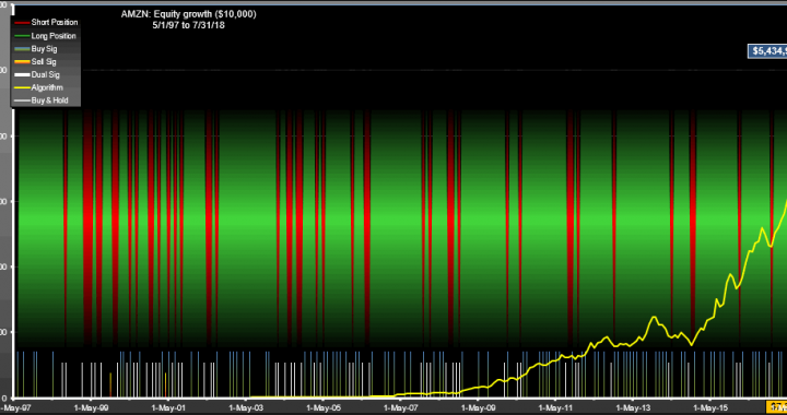
AMZN Equity

AMZN (Amazon) Signals – Monthly

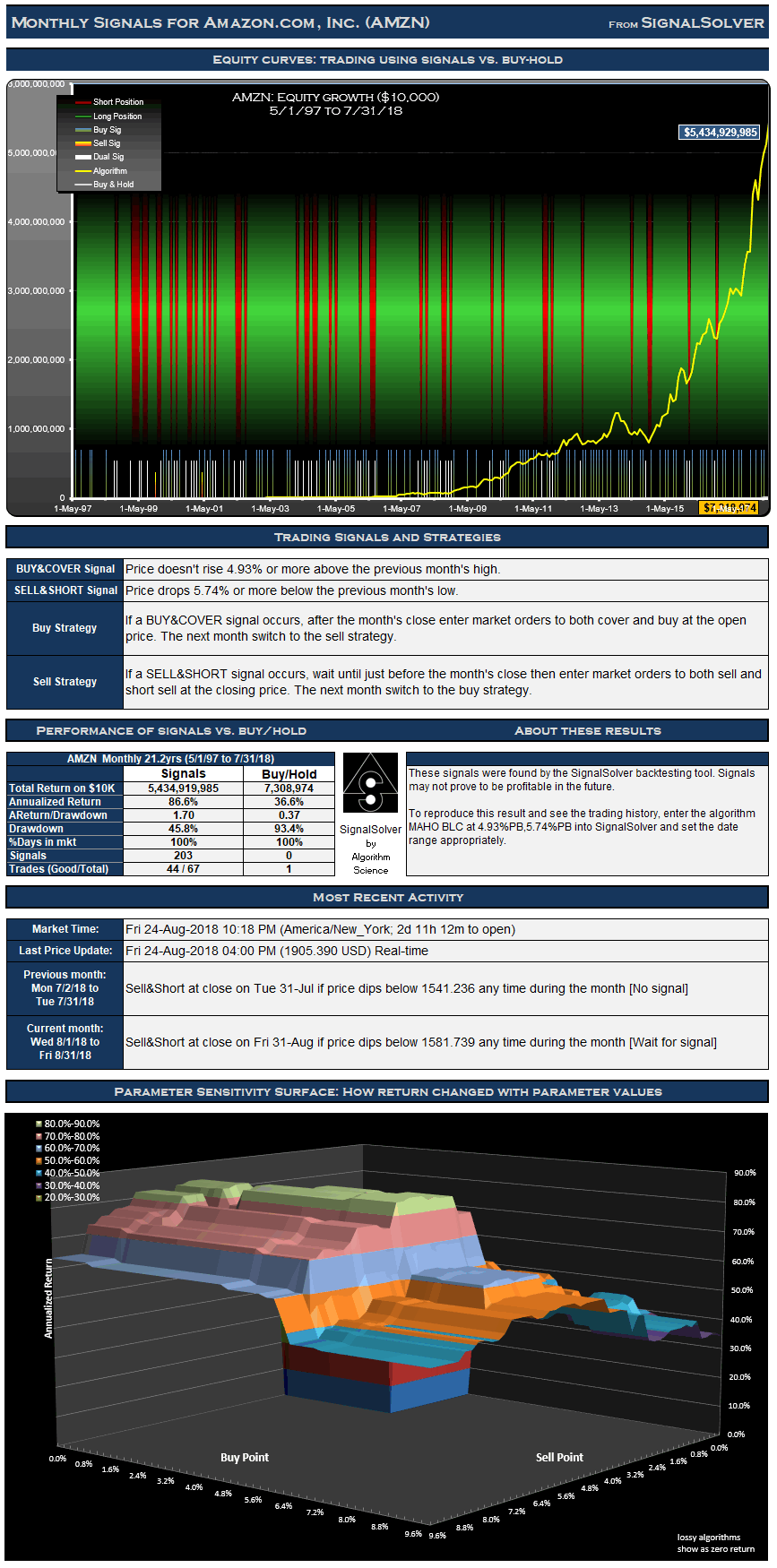
From Jul 2008 to Aug 2018, these trading signals for Amazon (AMZN) used as directed would have performed around 744 times better than buy-hold.

AMZN Signals Monthly

For the 255 month (21.2 year) period from May 1 1997 to Jul 31 2018, these signals for Amazon.com, Inc. (AMZN) traded long and short would have yielded $5,434,919,985 in profits from a $10,000 initial investment, an annualized return of 86.6%. The long-side profit (buy/sell only, no shorts) for the signals was $462,171,488, an annualized return of 66.1%. If you had bought and held the stock for the same period the profit would have been $7,308,974 (an annualized return of 36.6%). The trading style was Long & Short, meaning that you would be long or short the security at all times.

For this type of strategy, not every signal is acted upon and signals are often reinforced. If you are long in the security, buy signals can be ignored, for example. Similarly if you are short you can ignore sell signals. For this particular AMZN strategy there were 150 buy signals and 53 sell signals.These led to 34 long trades of which 22 were profitable, and 33 short trades of which 22 were profitable.

This is a monthly strategy; monthly OHLC data is used to derive all signals and there is at most one buy and sell signal and one trade per month. Drawdown (the worst case loss for an single entry and exit into the strategy) was 46% vs. 93% for buy-hold. Using drawdown plus 5% as our risk metric, and annualized return as the reward metric, the reward/risk for the strategy was 1.70 vs. 0.37 for buy-hold, an improvement factor of around 4.6

The MASC BAO Trading Strategy

Finding MASC BAO strategies on randomly selected stocks

The MASC BAO trading strategy frequently shows up in the top ten backtests. It has the distinction of being the strategy used in the most profitable backtest SignalSolver has ever found--AAPL Monthly MASC BAO which would have generated over $400 Billion from $10,000 invested.

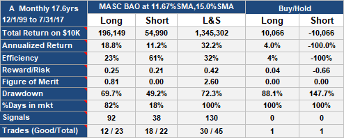
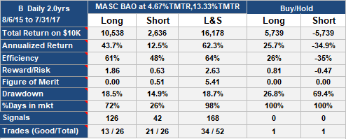
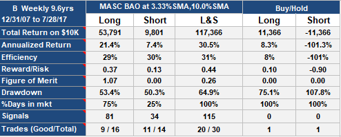
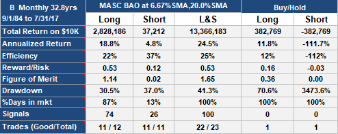
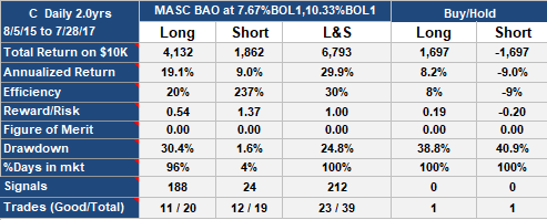
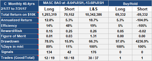
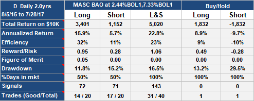
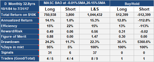
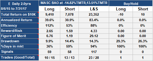
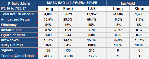
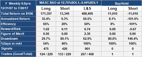
Here we look for MASC BAO strategies which beat Buy/Hold for stock symbols A through F (i.e. an arbitrary selection) using backtests run against daily, weekly and monthly data for each stock. The point of the exercise is simply to show that you can usually find a MASC BAO algorithm that beats buy or short-hold. Here are the results:

MASC BAO backtest results

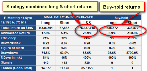
Each table shows the difference between the buy-hold returns and the returns from the MASC BAO strategy. Strategy returns are shown in three parts, those for the long only, short only and combined long&short (L&S). Also of interest are the Reward/Risk numbers (higher is better).

You can see that for all 18 data sets, SignalSolver was able to find MASC BAO trading algorithms which beat buy-hold or short-hold. Many were significantly better, such as the 83% annualized return for E daily (vs 0% for buy-hold), however a few were only marginally better such as the 15.3% for D weekly (vs. 12.8% for buy-hold).

More about the MASC BAO strategy

MASC BAO roughly follows a "buy the dips but sell at the first sign of trouble" methodology. The MASC BAO strategy for the Percentage Band is this:

  1. A BUY signal occurs if, in a given period, the price fails to rise a fixed percentage above the last sale price.
  2. A SELL signal occurs if the price goes below a fixed percentage below the median price (i.e. half H+L) of the previous period.
  3. A sell signal turns a bullish position to bearish at the open of the subsequent period.
  4. A buy signal switches a bearish position bullish at the close of the period.
  5. You only respond to one signal per time period.

For example, if the last sale price was 100, a buy signal for [MASC 10% PB] would occur if the price in a given day, week or month failed to go above 110. This could be dangerous if you were trading short or long and short. If you were short and the price broke out to new highs, there would be no buy (cover) signals and you would lose all if the price went to double your short sale price. If you were just trading long, you would be simply be locked out of a bull run.

For other bands, the percentage value is calculated on the band in use and added into the reference (in this case last sale price on buys, median price on sells), as described here. Interestingly, only 4 bands emerged from this study: SMA (Simple moving average), TMTR (Trimmed mean of the true range), Bol1 (Bollinger band 1) and the PB (percentage band). Other bands often gave good results, but these four bands gave the best results.

As always, good backtest results don't necessarily translate into future profits for any trading strategy.

Settings

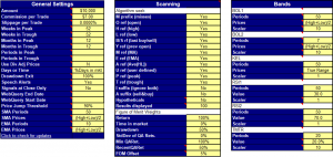
If you care to reproduce these results, here are the settings:

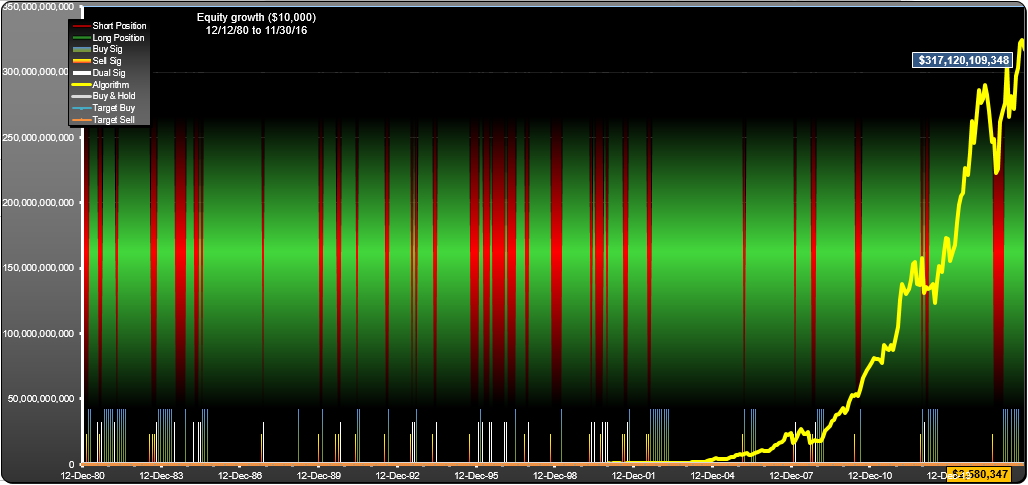
AAPL $31,000,000 trading strategy, equity curve

AAPL $31,000,000 Algorithm

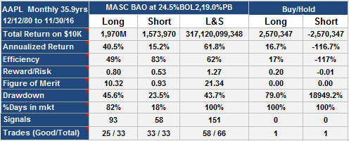
This AAPL trading strategy would have given a return of $31,712,009 for every dollar invested in December 1980. That's 123,000 times better than buy-hold, with nearly four times the annualized return (61.4% vs 16.7% for buy-hold) and roughly half the drawdown which  amounts to over six times better reward/risk than buy-hold.

AAPL $31,000,000 trading strategy: Table of results

AAPL $31,000,000 trading strategy: Table of results

This is a variation of the MASC BAO algorithm which I have published before,  except this time the buy point is related to a Bollinger Band instead of just the sell price. I found it using SignalSolver.

Here is the strategy:

Description of the AAPL $31,000,000 trading strategy

Description of the AAPL $31,000,000 trading strategy

Â

In this case the Bollinger band is the 7 period StdDev of median prices (monthly (H+L)/2), and the band is built around the last sell price, not the usual method of building it around a moving average. A little unconventional but it worked wonderfully. Algorithms with buy signals based on sell price often get stuck, but this one didn't. Sell signals were based on a raw Percentage Band built around the monthly median (H+L)/2 prices, just like the original version of this.

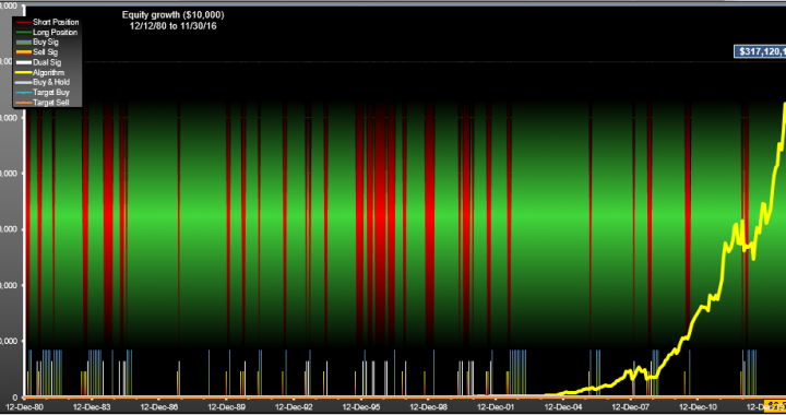
Here is the equity curve:

AAPL $31,000,000 trading strategy, equity curve

We are looking at quite a bit of reinforcement on buy signals, but sell signals tend to come in ones or twos. There are some dual signal months but not too many. Dual signals will trigger a trade for this algorithm.

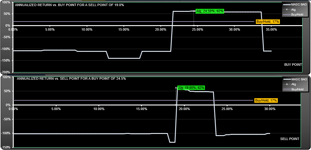
Moving onto the scans, you can see that there is a single area of profitability:

Annualized return vs. buy and sell point for the AAPL $31,000,000 trading strategy

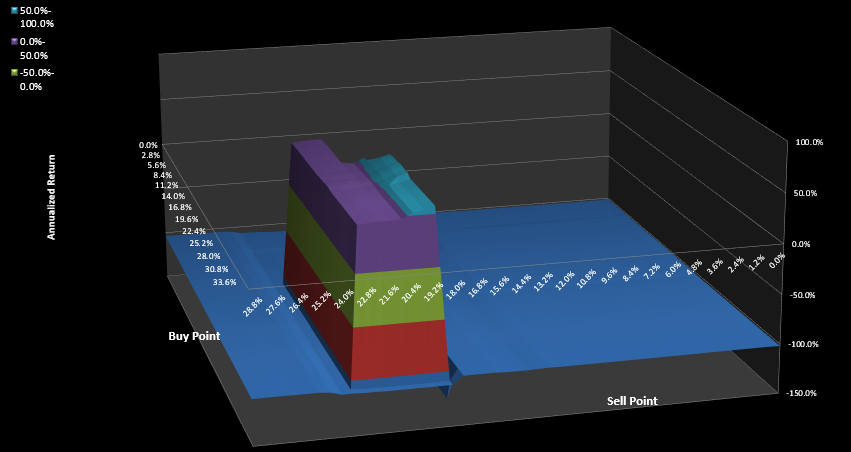
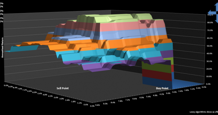
Getting the buy or especially the sell point wrong would have led to a complete loss, as this algorithm was run Long and Short (you were either long or short at all times). Here's the entire parameter surface, for completeness:

AAPL $31,000,000 trading strategy, parameter surface

A bit of a steep sided mesa, but a reasonably large plateau.

Since I found it in June, the algorithm has added about 3%, but it hasn't traded and is still long.

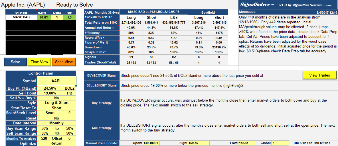
AAPL MASC BAO Update Aug 4th 2017

The algorithm has added around 40% since publication in Dec 2016, return on $10K would now be $432,155,847,777 . There have been no signals or trades and the position remains long.

AAPL Monthly Trading Algorithm MASC BAO $432,155,847,777 return for $10K initial investment, update 8/4/2017

AAPL Monthly Trading Algorithm MASC BAO $432,155,847,777 return for $10K initial investment, update 8/4/2017


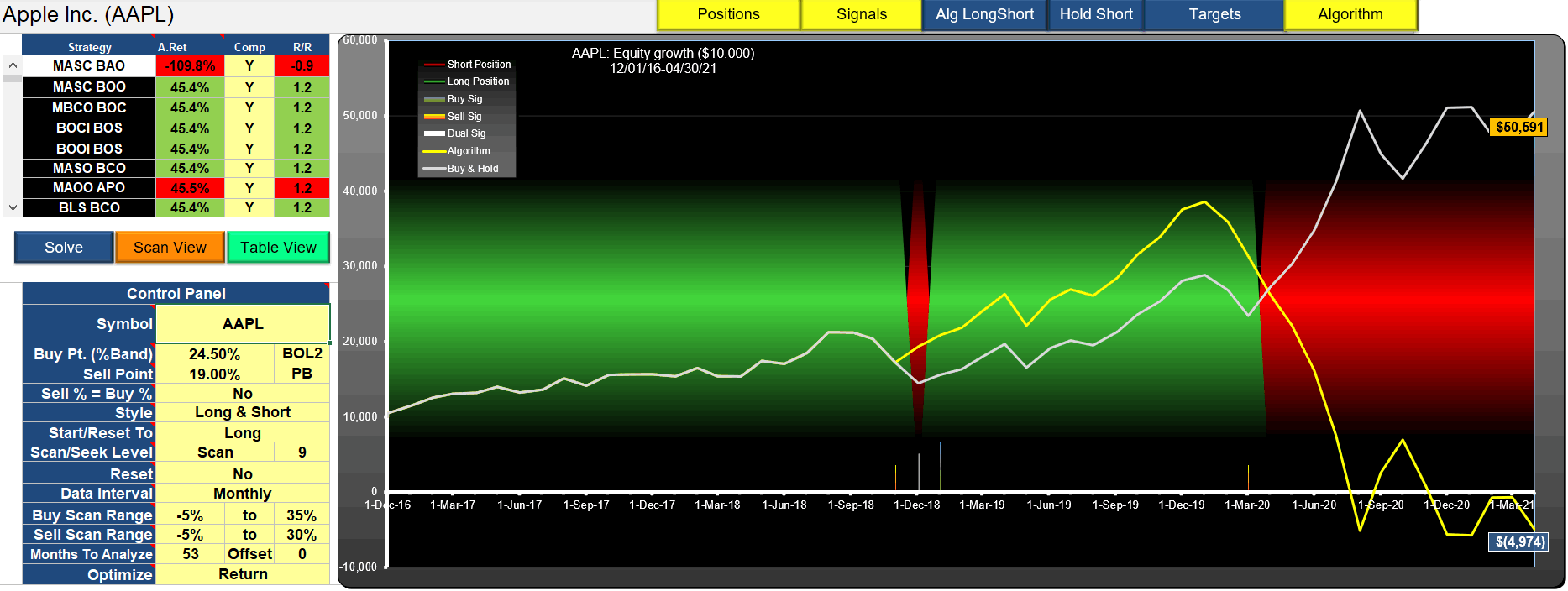
AAPL MASC BAO Update 5/4/2021

Just to round this out, the algorithm finally hit the dust in Aug 2020 making a total loss. Here's how it performed since its original publication in 2016. A mixed bag really, It kept you on the right side and did around 30% better than the underlying until about 3 years after publication, then broke down.  Like all algorithms based on backtests, they work until they don't. And you can't predict when the end will come.

In case you are wondering, re-parameterizing would have helped. A sell point of 27.28% or greater would have given you the same result as buy-hold, but without trading, so not terribly meaningful. But that's the best possible outcome for this algorithm over the last 5 years, a 45% annual return.

AMZN 20,000,000% total return

Over 500 times better return than buy-hold

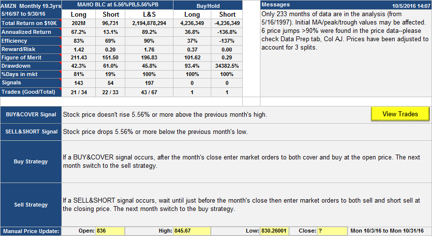
In the time frame May 16th 1997 to Aug 1st 2016, this strategy gave a return of 88.9% compounded which amounts to over $219,000 for every dollar invested, that's 518 times better than the performance of buy-hold which only gave $423.

This screenshot shows the strategy description and performance along with messages warning if something looks odd about the data. The data was checked and all the price jumps turn out to be real with the prices agreeing with prices from other sources.

amzn-m-table

The strategy used Long and Short investment style, so was always in the market long or short. The short side trades didn't do nearly as well as the long side trades, but well enough to boost the overall performance by a factor of almost 10. Also, the short trades had an efficiency of 69%, so for the short time that the strategy was short it did quite well.

Trading was at most once per month, trading a total of 67 round trips over the lifetime. 43 of these trades were good

This is a straightforward type of Percentage Band algorithm. Buy signals occurred in months when the stock price failed to rise, at any time, 5.6%  above the high of the previous month. This happened 143 times out of the 243 months of data. The buy was at the following month's open, but it only happened 34 times because the position was already long in most cases.

Sell signals occurred whenever the stock price fell 5.56% below the previous month's low at any time in the month. Usually, there was a buy signal the same month as a sell signal; there were 92 buy signal only months, 3 sell signal only months and 53 dual signal months. For this type of algorithm, if you are long you have to sell if a sell signal occurs, and you have to buy if a buy signal occurs when you are short. This is all explained in this video.

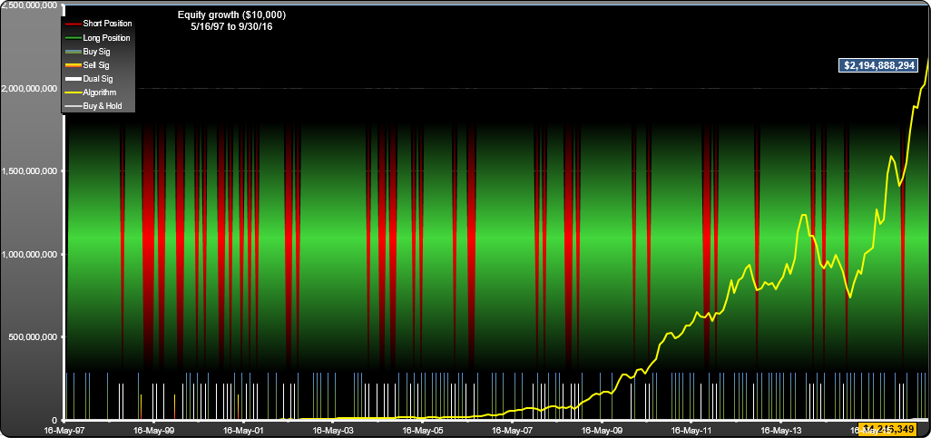
Here is the equity curve for the strategy, along with the signals and positions mapped out.

amzn-m-equity-curve

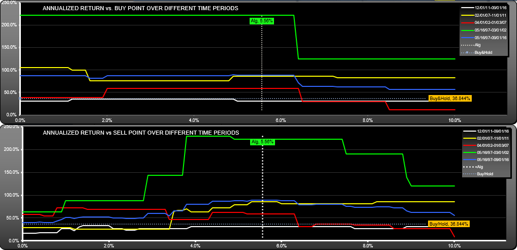
It looks as though the equity curve is still rising rapidly, however a closer look at the returns over different time periods (below) shows that most of the strategy gains occurred in the 1997 to 2002 time period. In fact, in the most recent quartus  (one fourth of the data, 2011 -16) the strategy did not quite keep up with buy/hold (31% vs 35.6% annualized).

amzn-m-longevity-scan

amzn-m-longevity

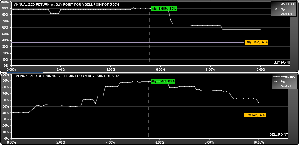
Looking at how changes in the parameters affect return, we see a broad area over which the buy parameters worked with a slightly narrower range for the sell parameter.

amzn-m-return-scan

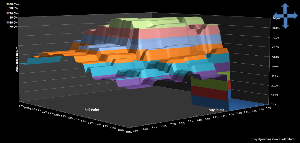
The parameter surface shows a nice large structure, showing that sensitivity to parameter changes was fairly low, but remember most of the gains were focused in the 97-02 timeframe.

amzn-m-return-surface-scan

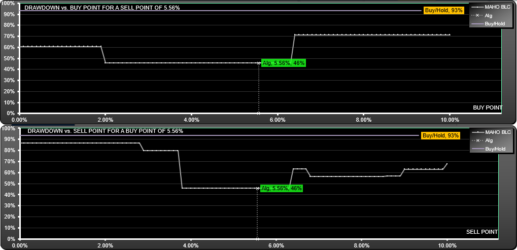
Drawdown for the strategy was much better than for buy-hold (46% vs 93%) and not overly sensitive to parameter change:

amzn-m-drawdown-scan

You can take a look at the buy-sell points on the trades list. As always, please be aware that there is no guarantee that this strategy will work in the future.

Recent performance

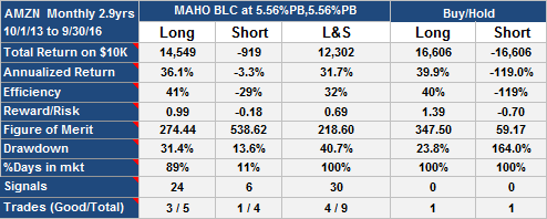
For the most recent 2.9 years, here is the performance table.

amzn-m-recent-table

There are not enough trades to make any firm conclusions about where the optimum parameters are now, but there is evidence to suggest that the buy point has pulled in somewhat. I suggest you download SignalSolver and optimize for different timeframes to get a feel for where the parameters might have moved to.

AAPL Trading Strategy (2)

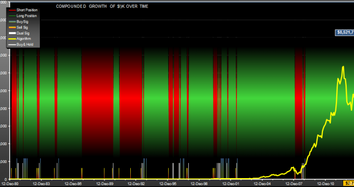
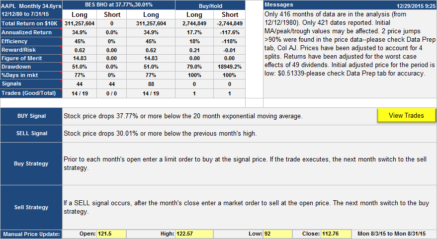
This is an interesting AAPL trading strategy for the period 12/12/80 through 7/31/15, which would have generated $8,521,705,763 in profits from $10,000 initial investment. Buy and hold would have generated $2,744,894 in profit in the same period. The cover and buy signals were generated when the stock price dropped 37.77% below the 20 month exponential moving average. Short and sell signals were generated when the price dropped 30.01% below the previous month’s high. Positions alternate between long and short. There were a total of 44 buy signals and 44 sell signals, you can see them at the bottom of the equity curve as vertical lines:
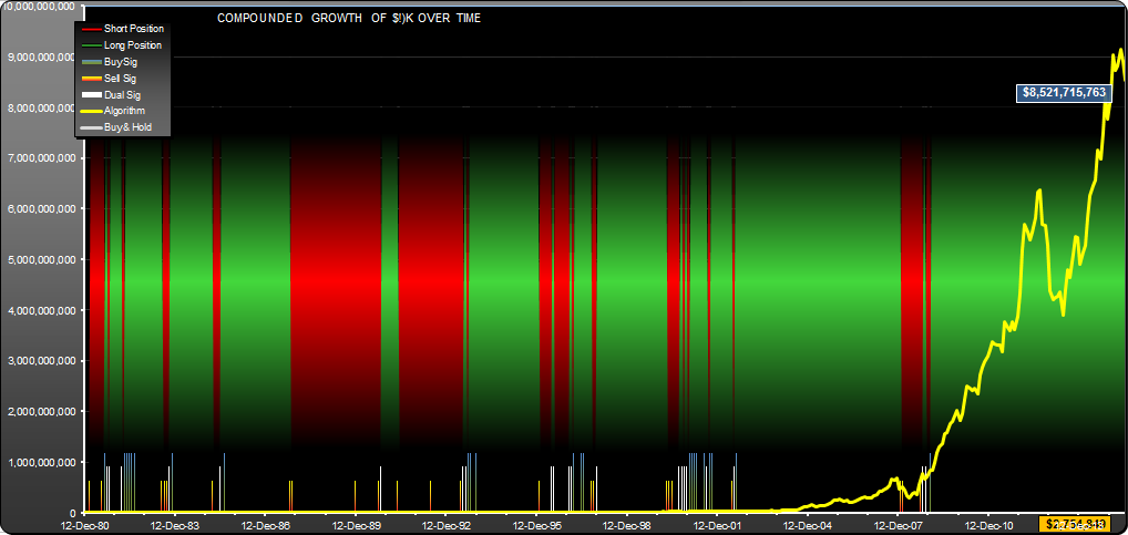
Blue/green lines are buy signals(23), red/yellow lines are sell signals (23) and white lines are dual signals (21). A dual signal always leads to a trade, but a buy signal would only lead to a trade if you were short, and a sell signal would only lead to a trade if you were long. So you can see there was some nice reinforcement on the signals.

The AAPL trading strategy and its performance

Selling/shorting was done at the next month’s open using market orders, while buying/covering was done when the signal arrived using limit orders. The green and red backgrounds behind the equity curve shows if you were long or short. The rules governing the strategy are shown in the performance table below. Signals are straightforward and response to signals is also simple.

Had you been lucky enough to have been following this AAPL trading  strategy, you would have needed to check in on it only once a month before the monthly open to place orders, a few minutes work. Only 39 of the orders placed actually executed as you can see from the Performance Table:
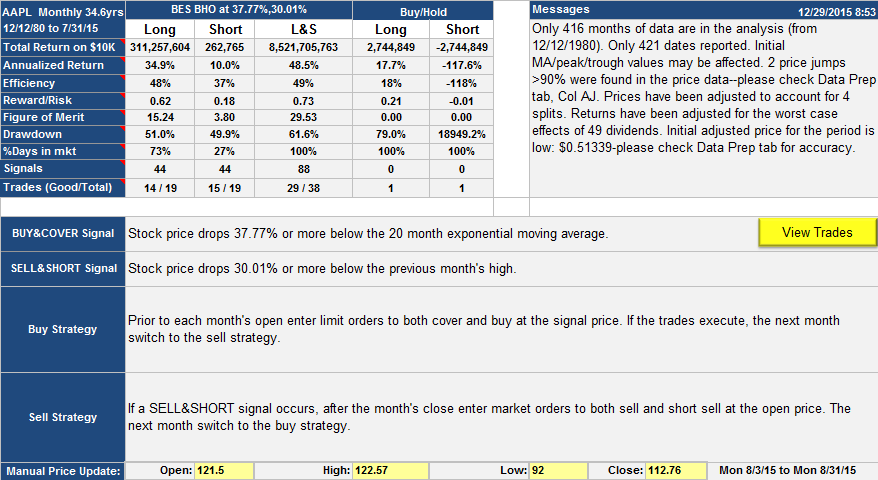
A few points about the Performance Table; In the Messages section you can see some warnings about the way the stock price moved. SignalSolver warns you about price jumps so you can check them out. In this particular case the jumps were for real–one drop in Oct 1987 (Black Monday), the other a drop in Sept 2000 as the dot com bubble burst.

The Performance Table also tells you how you would have fared if you had only played the long side (i.e. never gone short), or if you you had played the short side and never gone long. Clearly, playing both long and short (the L&S Column) sides was a better strategy in this instance, however you would have lost everything if the buy and sell points were not exactly as described.

Drawdown is the most you could have lost if you had entered a strategy at the worst possible time and then stopped using the strategy at the worst possible time. Notice the drawdown for the trading strategy was 61.6%. This may seem extreme, until you look at buy and hold drawdown of 79%.

Efficiency (relevant only for the long only and short only sides of the trading strategy) tells you the annualized return if you had invested at the same rate when you were not holding AAPL long or short. Its the annualized return divided by the % of time in the market. Reward/risk is the annualized return divided by the drawdown plus a 5% offset.

Figure of Merit is what the optimizing backtester uses to grade each of the algorithms. It can be set up to look for a rich variety of attributes like total return, drawdown or efficiency. In this instance we compared around 47,000 algorithms with about 13 million backtests optimizing min quartus return (see below).

The effect of parameter changes on return

Now we’ll take a closer look at the buy and sell parameters. Remember the strategy–buy if price drops 37.77% below the 20 month exponential moving average, sell if price drops 30.01% below the high of the previous month. Well, you need to look at the effect on return if you change those percentages. For that we look at the Scan Charts. First, the scan chart for Long and Short style.
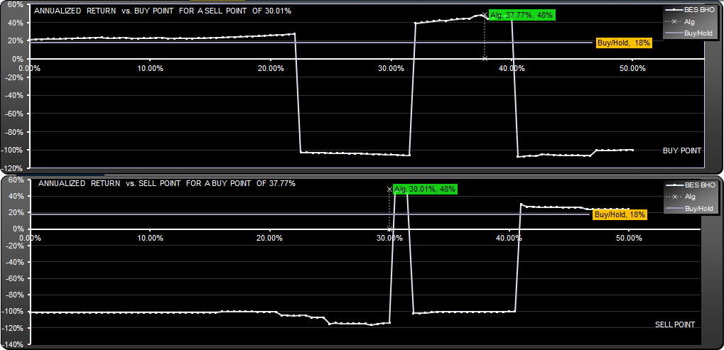
AAPL.M2 Scan LS

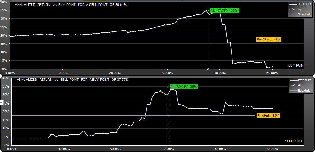
This shows that the profitable sell point range was very tight, between 30 and 32 %. Outside of this was a total loss. When you compare this with the scan for the Long only strategy, shown below, you can see the extreme downside risk of short selling a stock like AAPL. This makes the Long and Short strategy too risky to consider further, however the Long only strategy, with its 35% annualized return is still interesting, so we shall focus on that. Here it is:-
AAPL.M2 Table Long

and here is the scan result:

This is a much nicer scan result than the Long & Short strategy result. Focusing on the Long only scan, you can see from the top scan that if you had got the sell percentage right but used a buy point of 42%, then you would have done much worse. Similarly, if you had got the buy percentage right but used a sell percentage of 20%, again you would have reduced the profits considerably. On the positive side, if your sell point was 30.01%, you would have done better than buy hold for any buy percentage below 41.5%. Or, if your buy % was 37.77%, then you would have done better than buy-hold for or any buy % greater than 26%. But that’s not the whole picture. You can plot returns for every value of buy and sell point in the form of a surface plot:
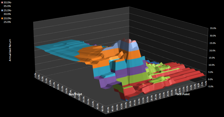
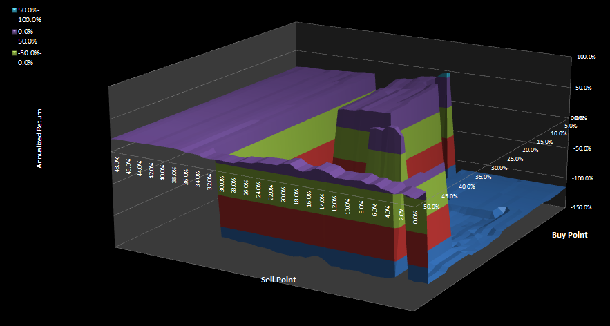
If you run SignalSolver, you can spin the surface plot around to take a good look for areas of low return were you could have got into trouble. The higher the hill, the more return you would have made if you were using those buy and sell points. You wanted to be high on the “hill” but not close to any cliffs as they imply risk.

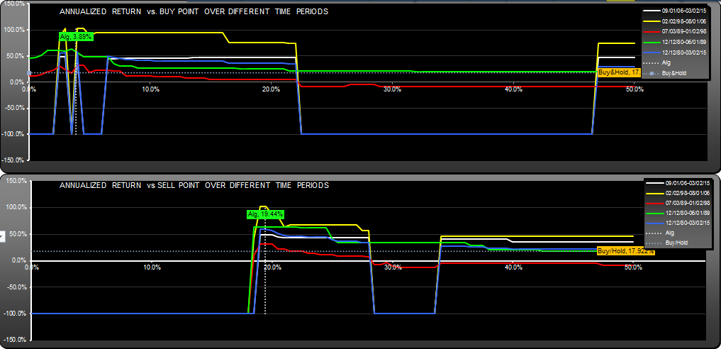
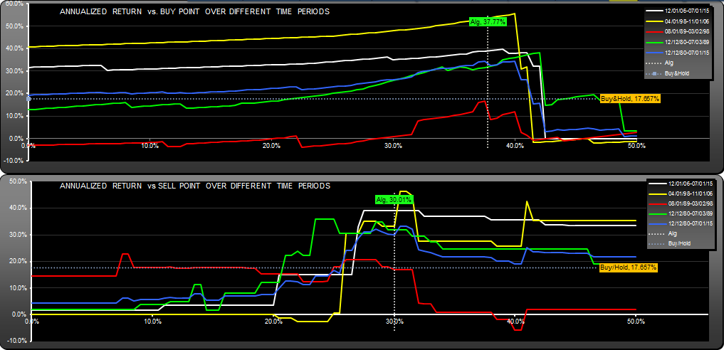
The next question is how did returns change over time for different buy-sell points? To answer this we use the “Life” Scan Chart:
AAPL.M2 Life Long

The Life scans are expanded views of the Scan Chart, in fact the blue line is exactly the same graph. The other lines show how the returns changed with buy and sell parameters for other time periods. Each time period is one quarter of the entire data set which happens to be 104 months (8.66 years) for this analysis. We call this a “quartus” (latin for one fourth) to avoid the ambiguous term “quarter”.

The trading strategy was found by setting up the SignalSolver backtester to search for the algorithm with the best “worst quartus”. Effectively, its looking for space under the Life scans. In this case, the annualized return for the worst quartus was 17% for the red period (8/1/89-3/2/98) while the best quartus was 53% ann. return for the yellow period (4/1/98-11/01/06). So while the return is nowhere near the highest returns I have found for an AAPL trading strategy, I think the (long only) strategy has better consistency and less sensitivity to the buy/sell parameters.

Note that the backtests assume a transaction fee of $7 per trade and slippage of 0%.

Here is the list of trades for the long side: AAPL.M2 Trades Long.

Andrew

Please note that there were errors in the original posting related to the short side of this algorithm. These have now been corrected (12/29/2015)

Update 10-20-2016

Strategy has followed buy-hold, losing about 4.8% since publication
AAPL Trading System (Monthly)

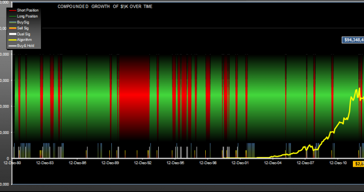
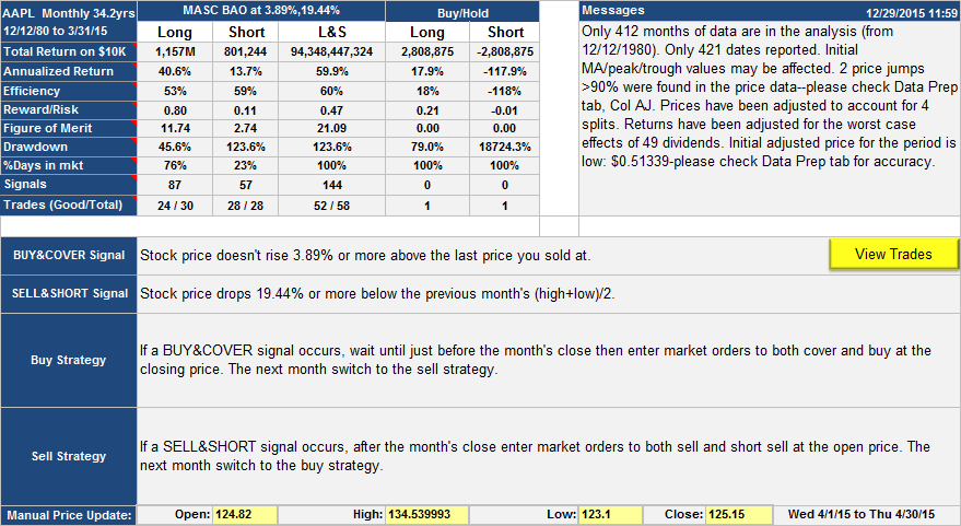
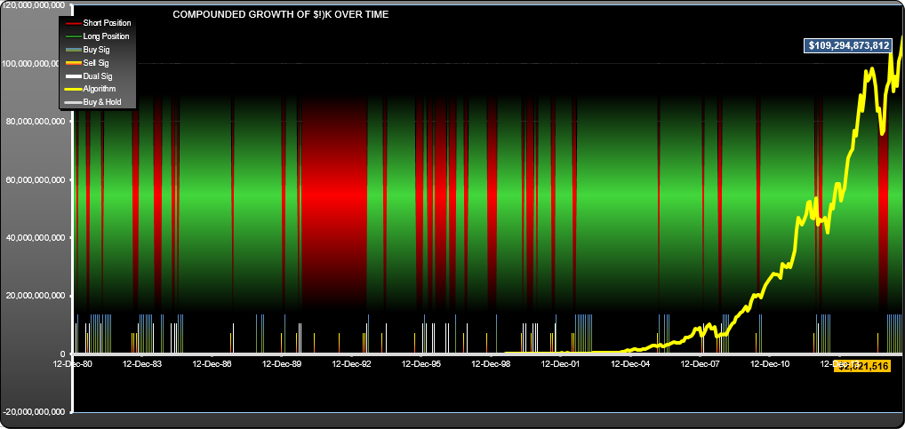
With $94 billion in profits (for $10K initial investment) this has one of the highest total returns I have seen for any algorithm.

It is an interesting study, but I wouldn't recommend it as a good system to trade moving forward. It is somewhat over-tuned, and the parameters are close to regions which would have failed. At one time the equity went negative and you would have required extra capital to satisfy margin calls. The algorithm uses the "last sell price" as a reference. This can lock up an algorithm if the stock price is trending, in this case starving it of buy signals if the buy and sell percentages were chosen wrongly.

That said, I've been watching it for a year or so and it has behaved itself. The one take-away that you might find valuable--if you are holding AAPL and you see that portentous 19.44% or more price drop in a month, maybe you should take heed and sell at the next monthly open. The 29 times this happened over the last 34 years, you could buy at a better price later on.

Notes: returns are compounded, commission was $7 per trade. Here is a list of trades: AAPL.M Trades

Note that the short side of the algorithm has a drawdown of 123%. If you look at the trades, you will see that this corresponds to a peak of $833,000 in Oct 90 and a trough of -$196,000 in May 91. This can happen on the short side of an algorithm, and would have led to expensive and quite possibly disastrous margin calls. The algorithm, however, recovered the following month when the stock price fell dramatically.  The long side of the algorithm made $1,066,052,956 with only $10K at risk.

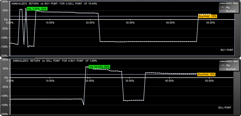
The scan shows how the return changes with choice of buy and sell point. We have chosen to show the peak, but better choices would have been in the center of the profitable regions.

These scans show how returns change with buy/sell point for different timeframes.

The scan shows returns for the entire buy/sell point space. High points are good, low points are, in this case, losses.

Please note that this post was edited 12/29/2105 to correct a calculation error on the short side of the algorithm.

AAPL Apple Trading Strategy (Monthly) Update 10/20/2016

Strategy returned 11%, buy-hold -5%

AAPL Trading Strategy (M) Update 10/20/2016

AAPL Trading Strategy (M) Update 10/20/2016

AAPL Trading Strategy: Equity curve as of 10-20-2016

AAPL Trading Strategy: Equity curve as of 10-20-2016

GOOGL Trading Strategy (Weekly Setup)

Algorithm for GOOGL based on monthly OHLC data and requiring monthly setup.

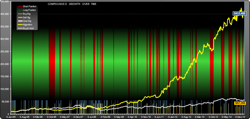
GOOGL.M Time

Buy signals around 3 times more frequent than sell signals, some overlap (dual signal months shown as white lines). 80% long, 20% short. Algorithm showing flattening out of performance in recent months.

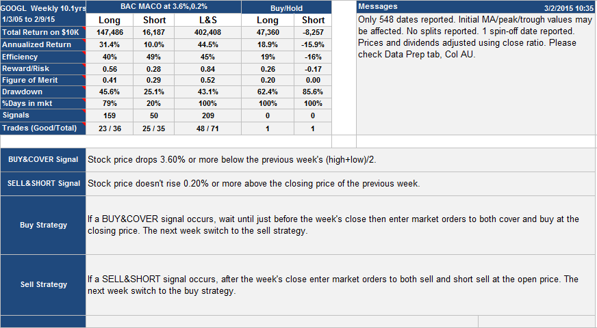
GOOGL.M Table

GOOGL.M Performance table and strategy description. Showed about 3 times the reward-risk of buy-hold. Strong bias to buy side (as is appropriate for upward trending stocks), clearly shown in signal count and %days long vs. short.

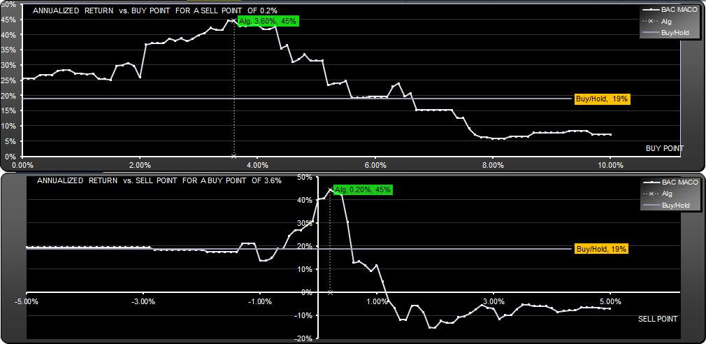
GOOGL.M Scan

Return vs. parameter for buy and sell parameters. Buy side is reasonably insensitive. Sell side seems more highly tuned, however algorithms of the "misses target" type often have this characteristic of being tightly clustered around zero.

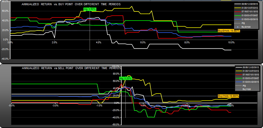
GOOGL.M Life

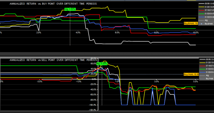
The life chart shows parameter sensitivity for different time periods. All timeframes beat buy-hold by a decent margin.

GOOGL.M Surface

GOOGL Surface chart showing how return changed with buy and sell parameters.


Update 10/20/2016

GOOGL Trading Strategy Weekly Update Oct 19th 2016

GOOGL Trading Strategy Weekly Update Oct 19th 2016

MU Trading Strategy (Monthly)

Micron Technologies monthly trading strategy, 46% Annualized Return, 25 years

Please note, this post was edited Jan 6th 2016 to correct an error in the short-side calculations. The original post showed an annualized return of 57%, which was erroneous. Below are shown the corrected results for this algorithm.

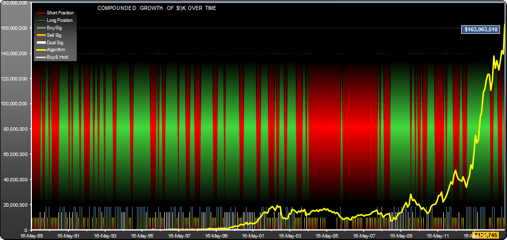
Micron Technology (MU) trading strategy base on monthly OHLC data. Would have returned $153,063,510 for a $10K initial investment. B/H returned $111,745 over the same period (5/16/89 to 2/2/15). Signals (at bottom of graph) generally show good reinforcement with occasional periods of confusion. Background red/green stripes show short/long hold periods

MU Monthly. Annualized return for this trading strategy was 46% vs 10.2% for buy/hold. Drawdown was a disconcerting 97.1% for buy/hold in Dec 2009, vs. 57% in Sept 2006 for the trading strategy. The price jumps reported were 50% drops in '87 and '00. The "user defined price" referred to in the strategy is the open price of the current month plus the high and low price of the previous month, divided by 3. Reward-risk was 6.7 times better than B/H using return/drawdown+10% as the yardstick.

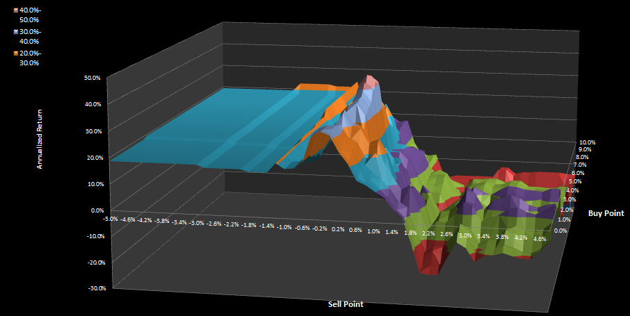
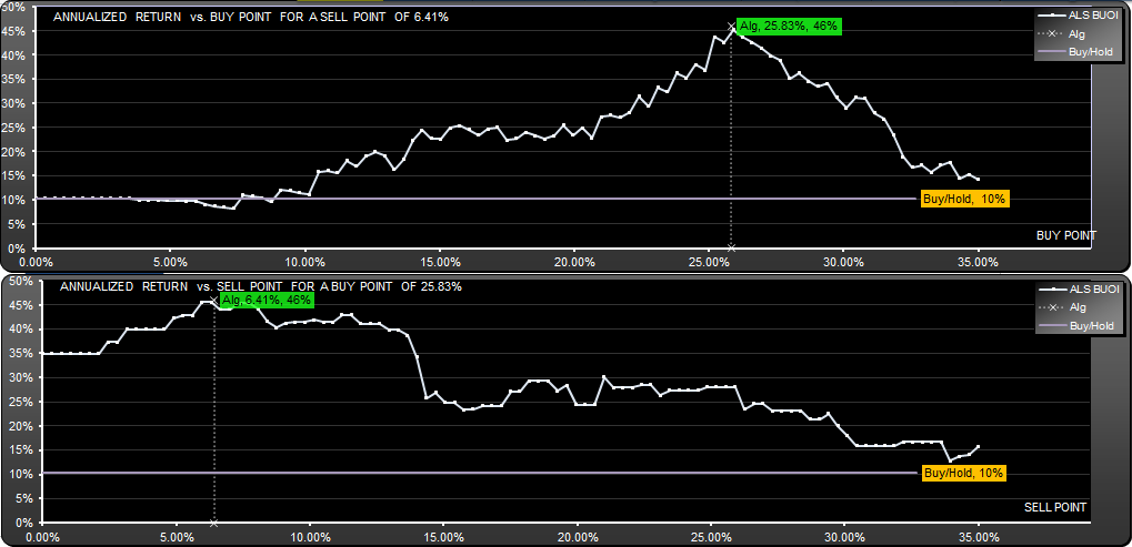
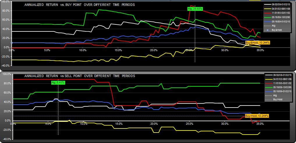
This graph shows the effect of changing the buy and sell parameters on the annualized return of the algorithm. For a buy point of 25.83%, all sell points 0 through 35% were profitable. For a sell point of 6.41%, all buy points 0 through 35% were profitable.

The life graph shows the return vs buy/sell points for different periods. The problem here is that the yellow graph shows that there was a period (5/89 to 10/95) with much worse return than the other periods. A more consistent algorithm over time would be preferable to the author, even if it had lower returns.

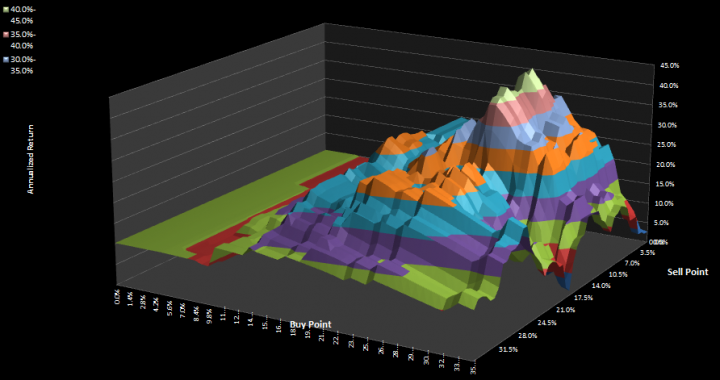
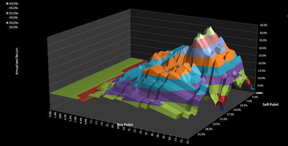
The parameter surface shows how the return changed over the whole parameter space. Cliffs and steep slopes are not good, but for this the drop-offs are reasonable.


MU Monthly, Update Jan 6th 2016

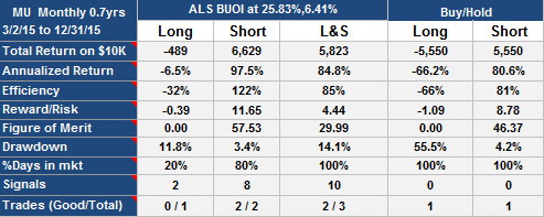
MU-M Table 1-6-2016

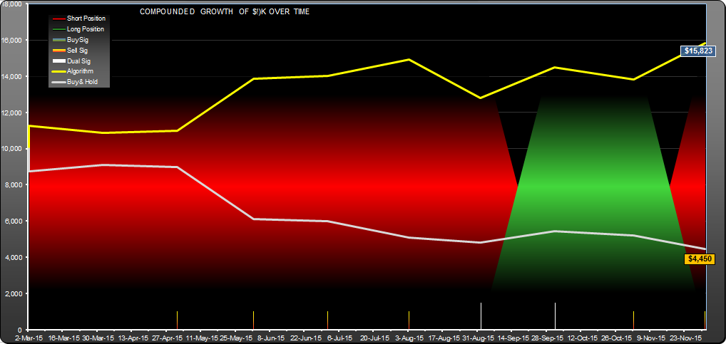
Since original publication, this algorithm would have returned 58%

MU-M Equity 1-6-2016

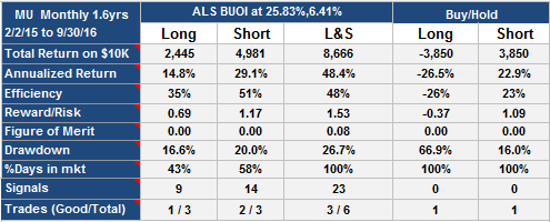
MU Monthly Trading System, Update 10/19/2016

The strategy, since publication in Feb 2015, has performed much better (86% return) than buy-hold and short-hold, with good drawdown. However, the optimum buy parameter for the period (16.45%) would have yielded a 151% return.
MU Monthly trading strategy update 10/192016

MU Monthly trading strategy update 10/192016

Since 5/16/89 the strategy would have returned $279,572,374