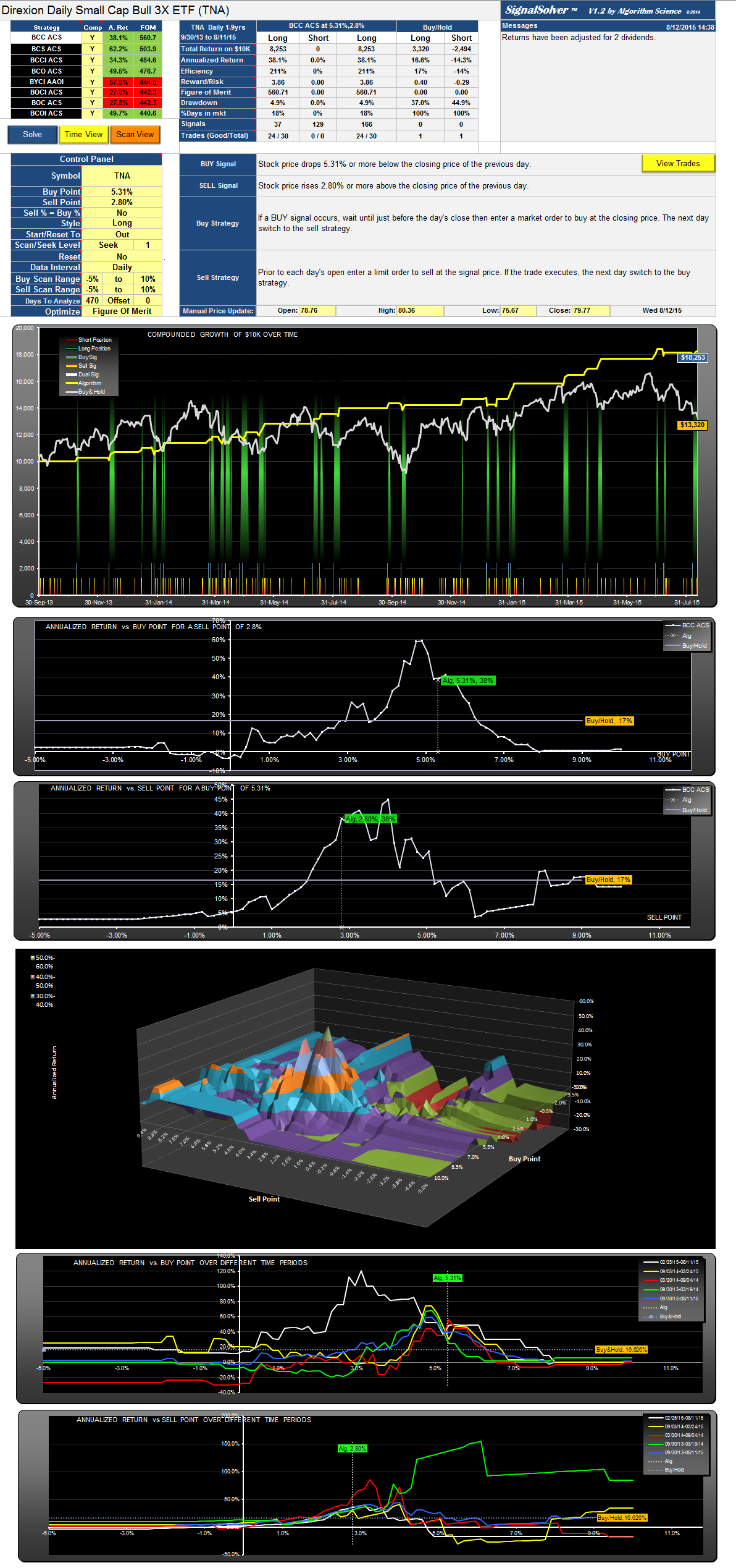
Another low drawdown trading strategy-TNA Direxion Daily Small Cap Bull 3X
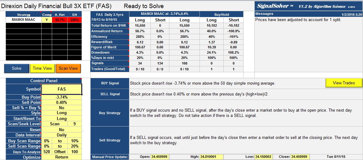
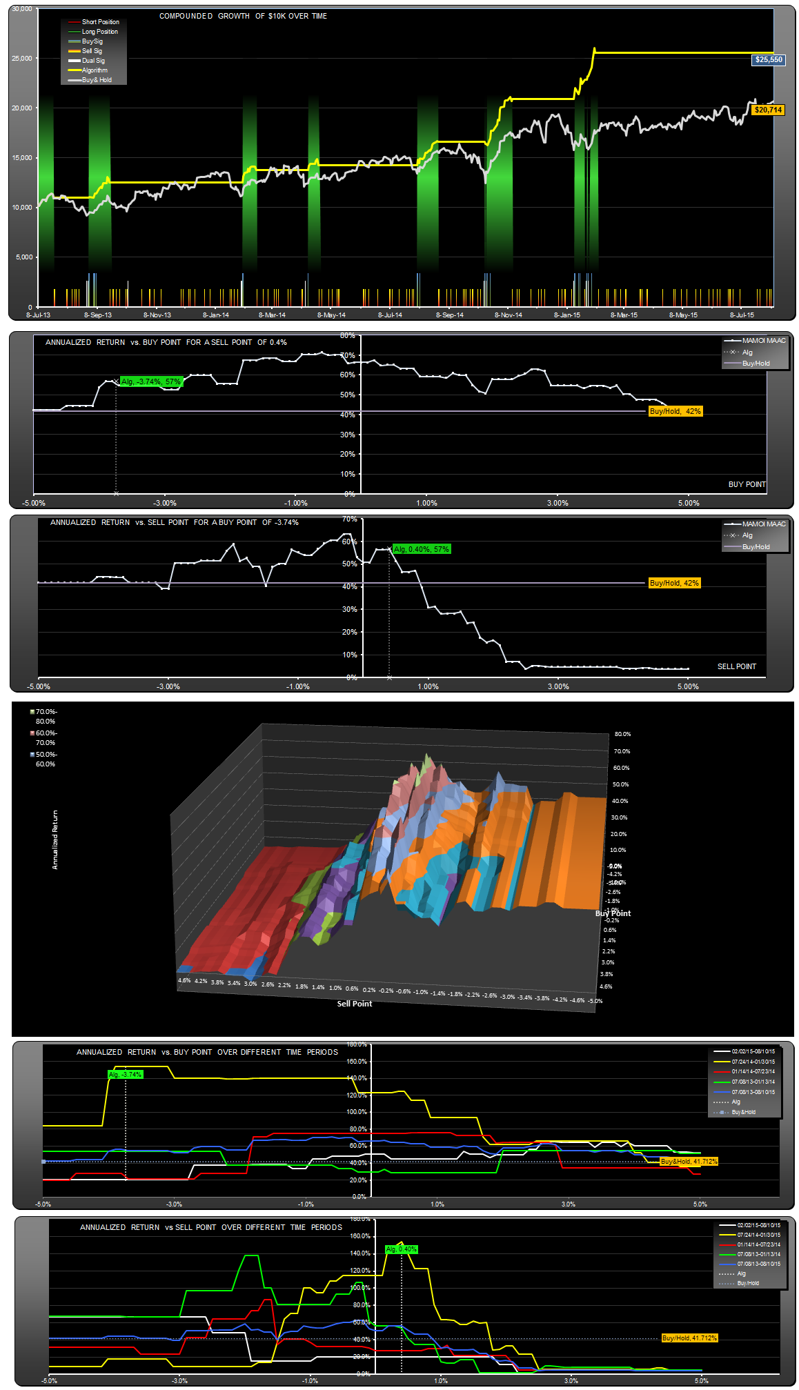
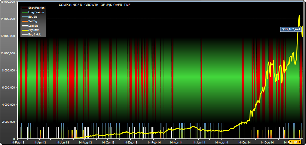
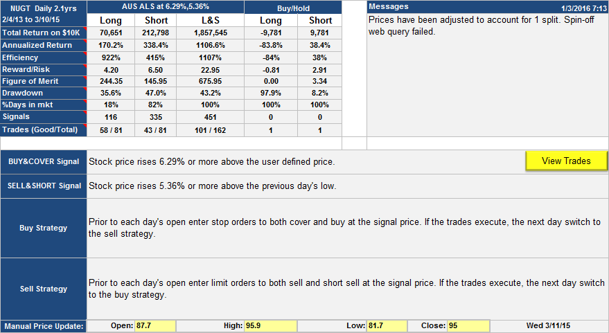
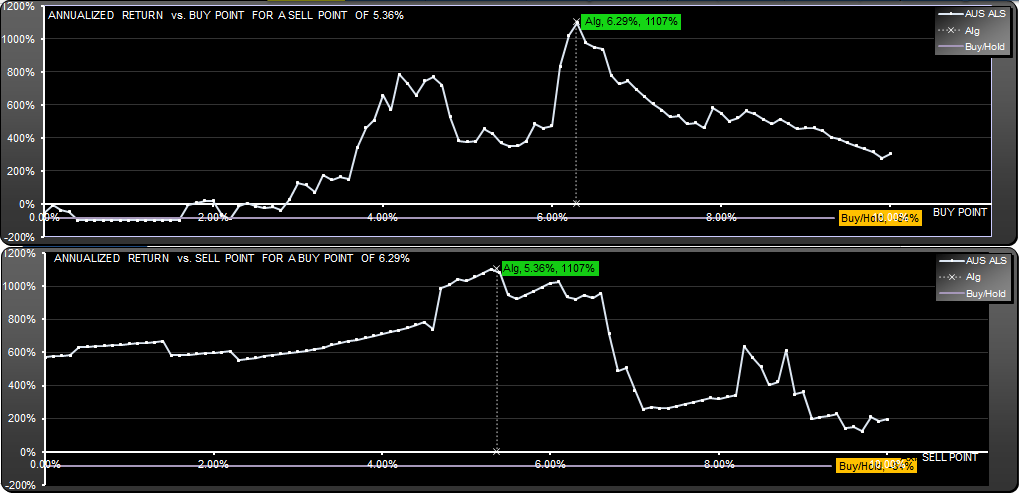
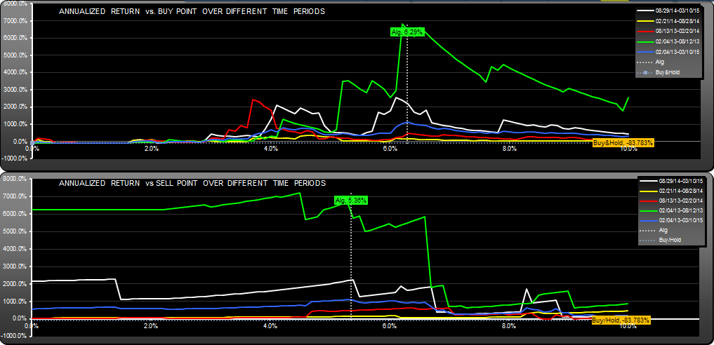
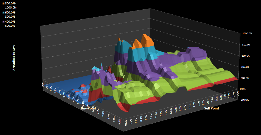
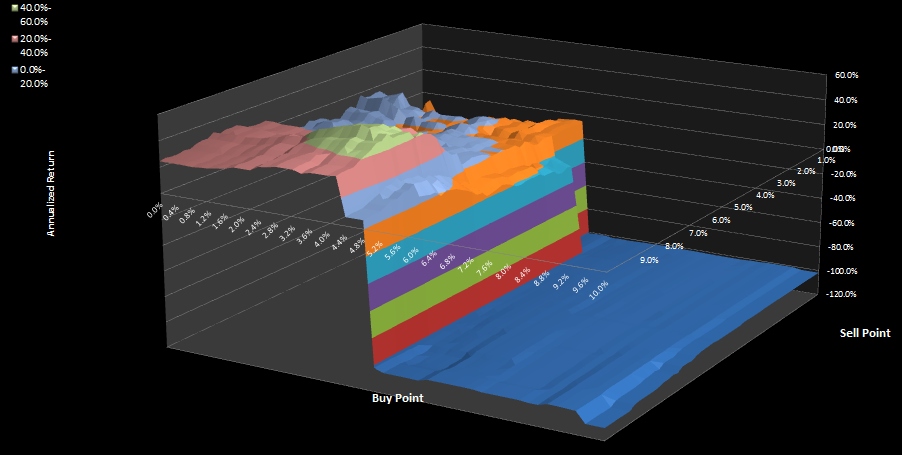
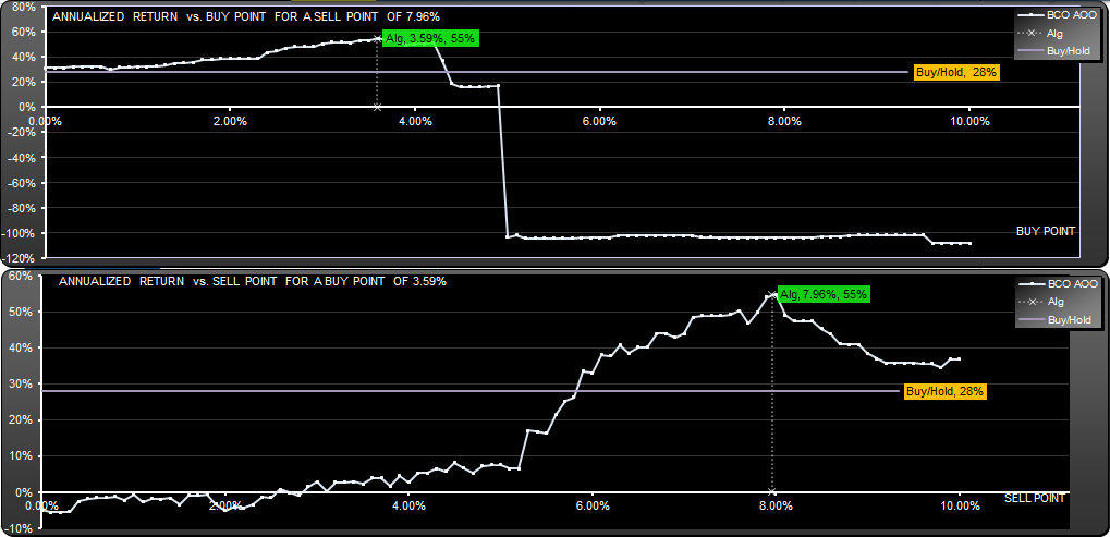
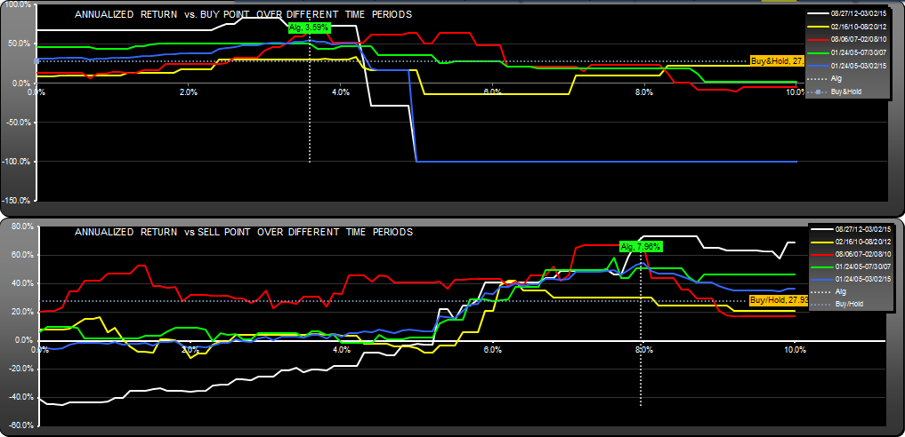
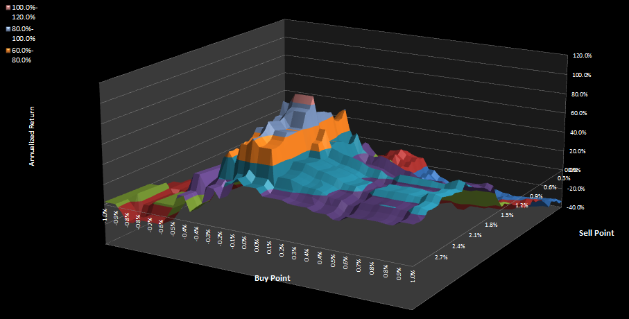
In the same vein as yesterday's FAS analysis, here is a low drawdown trading strategy for TNA, with daily intervention. Prasad had asked me to search for low drawdown strategies for a few of the triple leveraged ETFs, this being one of them. As with FAS, the algorithm was found by optimizing the SignalSolver backtest engine for drawdown (100% weighting), with a min QA return weight of 50% thrown in to get rid of all the zero trades-zero return hits. Period of the analysis was 1.9 years.
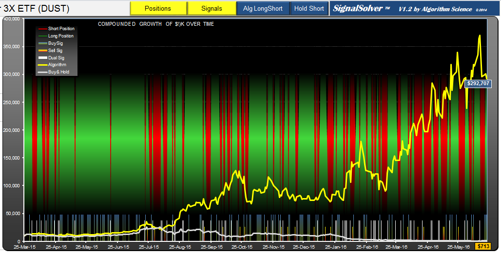
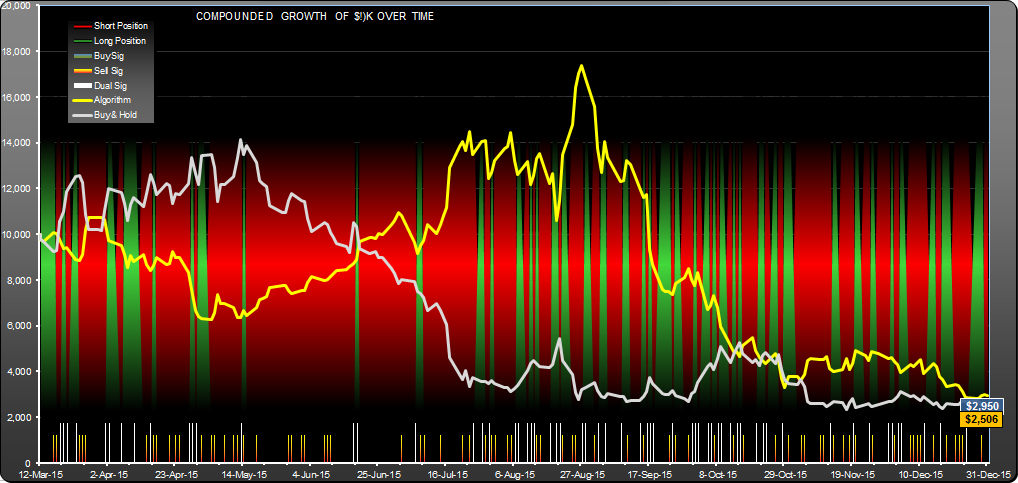
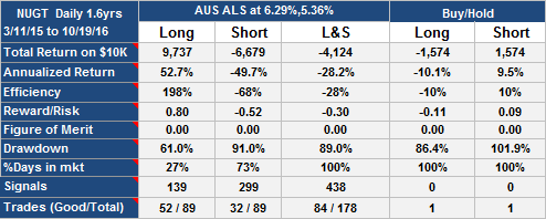
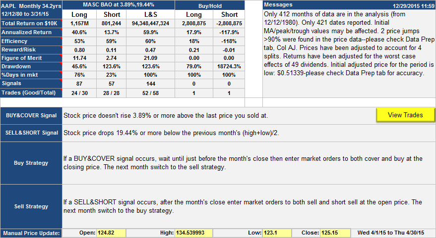
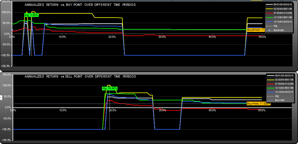
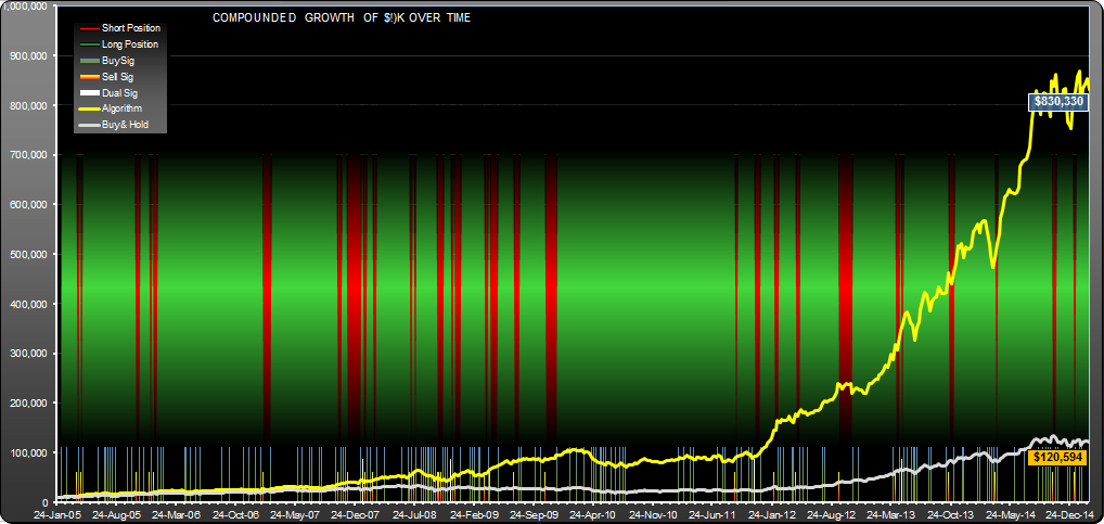
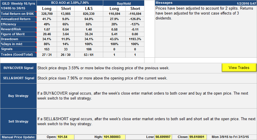
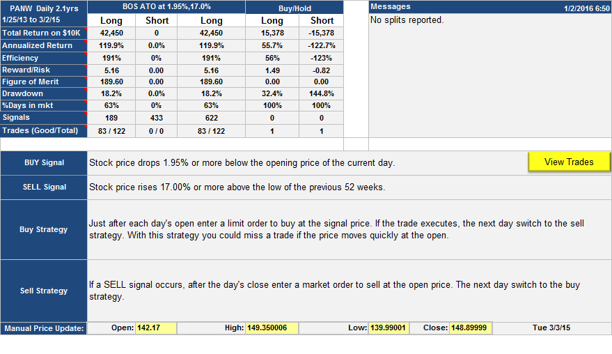
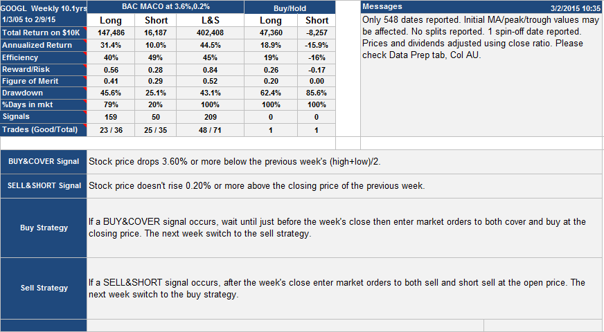
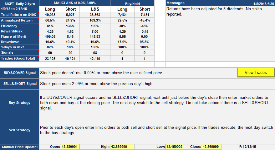
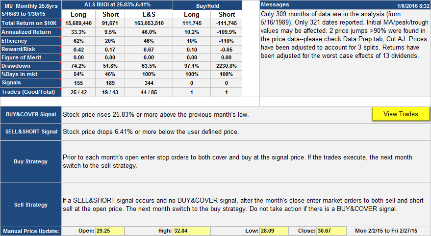
Again, the result had a low time in the market (18%), low drawdown (4.9%) and an annualized return which, while modest (38%), was better than the underlying ETF.
Andrew
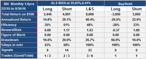
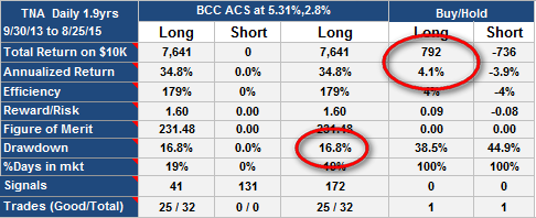
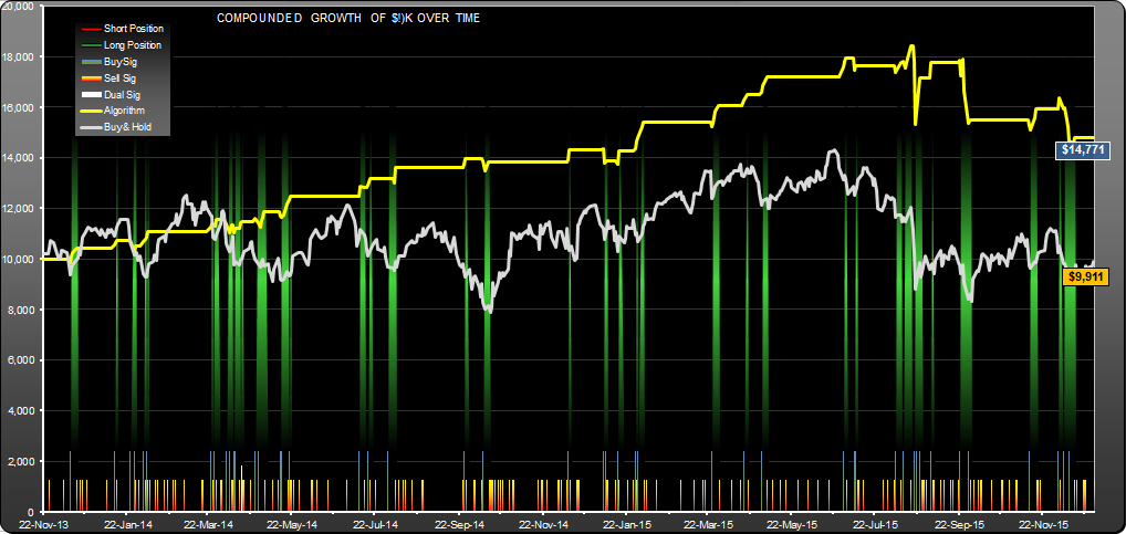
Update 8-26-15
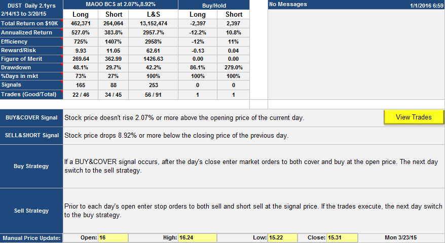
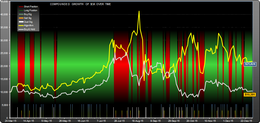
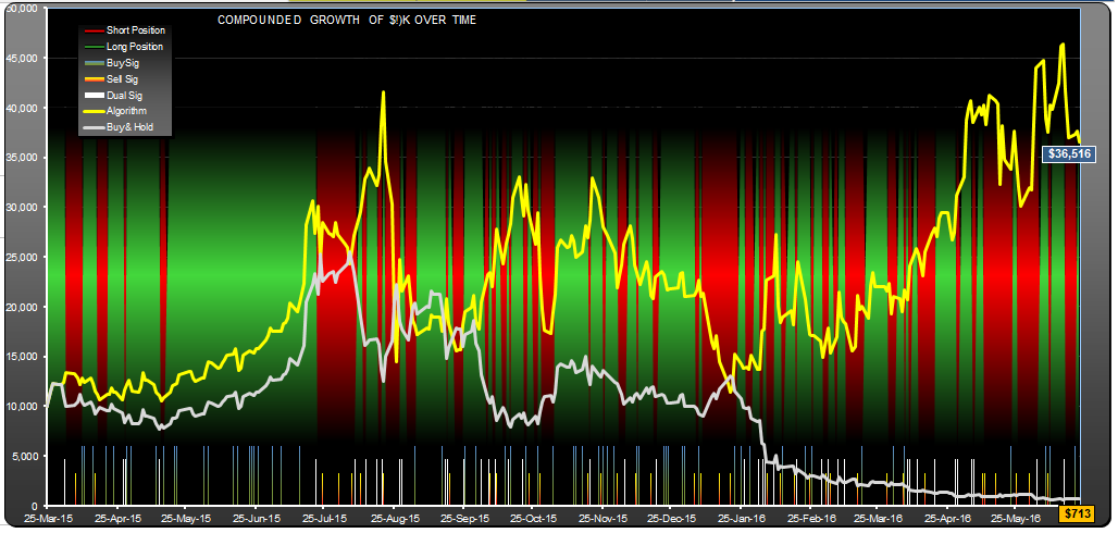
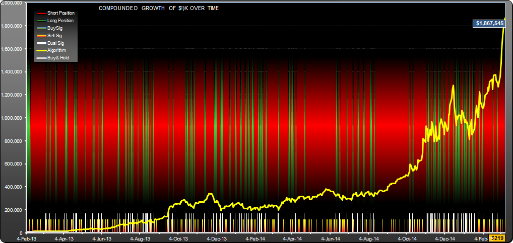
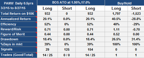
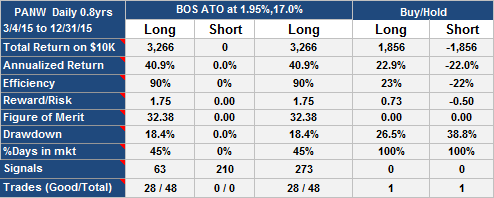
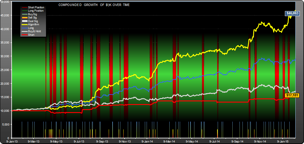
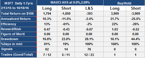
As per the table below, you can see the drawdown has jumped up to 16.8%. On the positive side, the differential in performance of the algorithm vs. the underlying TNA stock has grown.
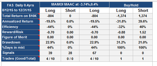
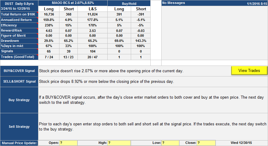
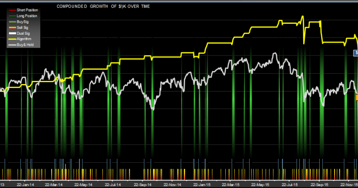
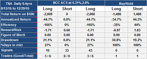
Update 12-30-2015
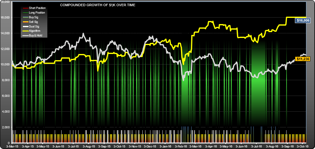
This algorithm peaked close to the day of publication, and has not done well since then:
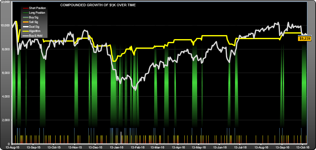
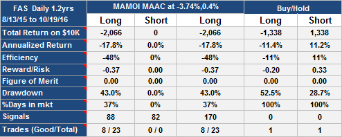
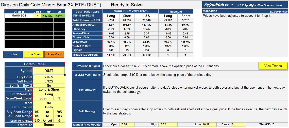
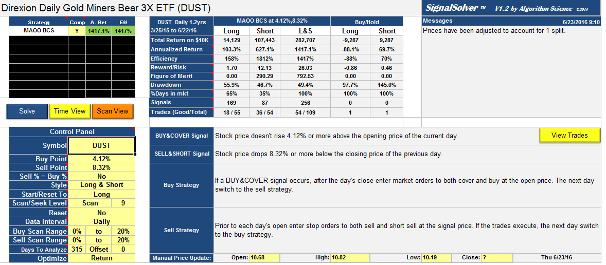
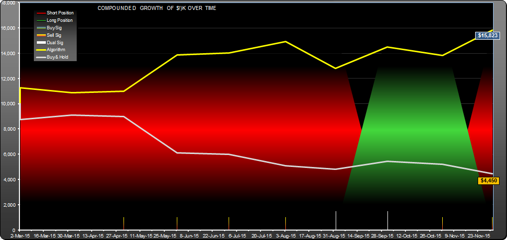
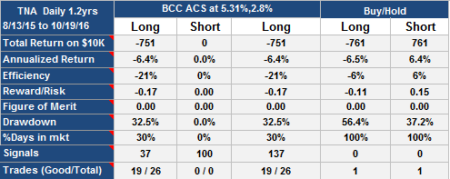
Update 10-20-2016
Slight improvement over last update:
TNA Trading System Update 10-20-2016