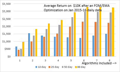
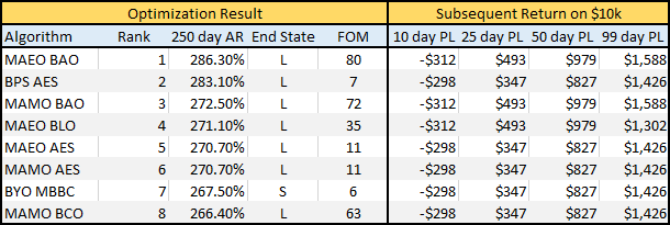
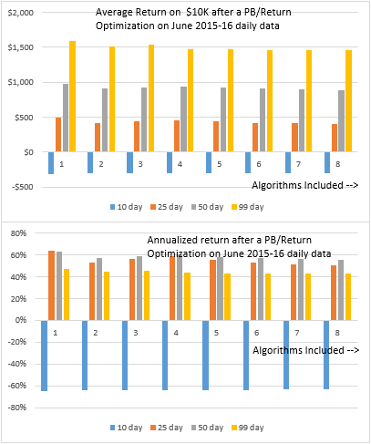
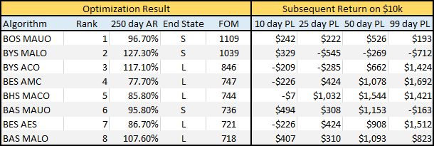
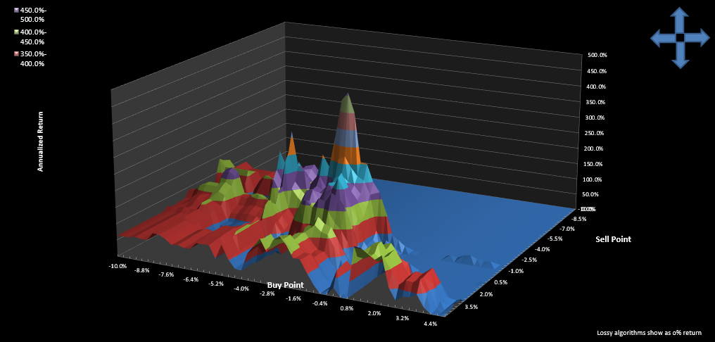
Multi-algorithm test results for NUGT (4 algorithms)

Multi-algorithm study results for NUGT DUST and X

Multi-algorithm study results for NUGT DUST and X

In the interests of scientific method, I'd like to continue the multi-algorithm study by discussing the worst results, those for X (United States Steel Corp. ), NUGT(Direxion Daily Gold Miners Bull 3X ETF) and DUST(Direxion Daily Gold Miners Bear 3X ETF). There was plenty of potential for disaster in these stocks, very large swings indeed. In fact, as you shall see, these often led to total loss of capital because the algorithms were run both Long and Short--if the stock price doubles and you are short, you are wiped out. All the results for the study can be found in the spreadsheets.

Multi-algorithm test results for X (United States Steel Corp.)

     Multi-algorithm test results for X (United States Steel Corp.)

Multi-algorithm test results for X (United States Steel Corp.)

While the September and Jan optimizations were almost all lossy, the Jun optimizations led to profits for the 50 and 99 day horizons, so overall, losses were fairly neutral. But the technique clearly failed to exploit the price movements of X. Look at the January buy-hold figures, there was plenty of room for profit on the long side, but harshly negative profits for the algorithms.  Similarly for Sept optimizations on the short side.

Multi-algorithm test results for NUGT

Multi-algorithm test results for NUGT (4 algorithms)

Multi-algorithm test results for NUGT (4 algorithms)

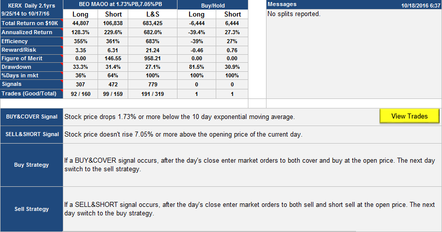
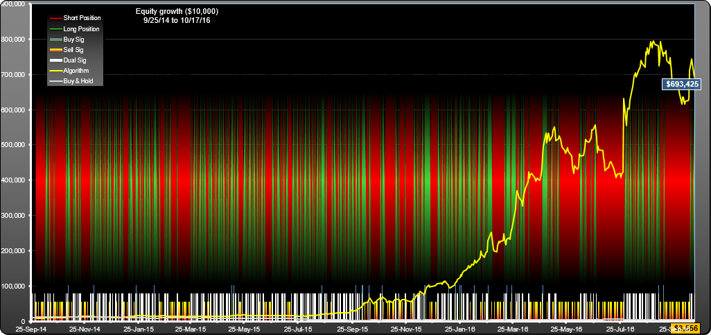
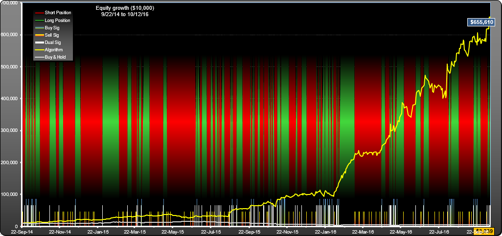
The January optimization results are the worst. 25 days into the test, 3 out of the 4 algorithms had gone belly up with a complete loss. Before the 99 days had elapsed, the fourth algorithm had also died off. Not that difficult to understand, though. For the Jan 15 to Jan 16 optimization period the stock price had dropped from $42 down to $3.50, consequently, all the algorithms had a strong short bias. Just at the start of the out-of-sample runs, the stock price started rising, from $3.50 up to $21 at the end of the 99 days. Oh well. On the positive side, most of these losses were offset by the June optimization results, so it  ends up being pretty flat returns overall, but sadly leaving these huge swings unexploited.

Multi-algorithm test results for DUST

Four algorithm result for DUST

Four algorithm result for DUST

While the June optimizations led to some decent exploits, the Jan results were again pitiful, stock price dropped from $1000 to $50, and the algorithms had a buy bias, so not a good result.


Multi-algorithm results for UWTI

Oil had a rocky year, lets look at how our multi-algorithm approach worked on an oil related stock, UWTI (VelocityShares 3x Long Crude Oil ETN). In this post, I'm just going to summarize the results:

Briefly, the method used is to run SignalSolver to find trading systems which worked for a 250 day period, then run these trading system against the data immediately following the 250 day period to see how they performed. This is known as out-of-sample testing as none of this following data is included in the optimizations.

The methodology is identical to my previous posts. If you need more details you can download the results spreadsheets, or download SignalSolver and run the optimizations yourself. I have omitted the result for the Return optimization on the PB band this time because I think we have established that the Figure of Merit optimizations usually work better. They do here.

The idea is behind multi-algorithms is that using a single algorithm is risky, but running multiple algorithms at once averages out your risk and leads to more consistent and more efficient (since you are sometimes out of the market) results. Here, we averaged over the top 4 algorithms for each period.

You can see that the multi-algorithmic approach gave very good results for the 25 day (5 weeks of trading) and 50 day runs. If you look at the buy-hold profile you can see that you would have had a rough time guessing long and short entry and exits to get the same results. Not saying it couldn't be done, but using the multi-algorithmic approach would have given nice returns for UWTI with absolutely zero guesswork. And its based on sound numerical analysis, not hunches and tweets. Is anybody listening? 🙂

Multi-algorithm analysis for FB (Facebook)

Today, I'll just throw out some more results from the multi-algorithmic testing I've been doing with SignalSolver. This time for Facebook (symbol FB). This is a stock which moved a lot in the time-frames used in the study. Could SignalSolver correctly predict and capitalize on these price movements? Let's see...

Optimizations for June 2015 through June 2016

As described in the methodology and the AMZN results, two optimizations were run on the June 2015 through June 2016 stock price data, one which rewarded raw returns using the Percentage Band, the other which rewarded more consistent returns and using the EMA band. First, lets look at Buy-hold performance for the subsequent periods:

Now lets see if the algorithms were able to exploit these price movements.

Results of the Return Optimization:

Now, the results for the Figure of Merit optimizations:

and the multi-algorithm averages:

One difference to note is that the return optimized algorithms were started out in a long state (because the End State vote indicated Long 7 to 1), whereas the FOM optimized algorithms were started out of the market because there was no good consensus. Accordingly, these returns would have been realized with lower capital.

Jan 2015 to Jan 2016 FOM Results

Here's the buy-hold results:

A pretty dramatic rise at the end of Jan 16. Luckily, all the algorithms were started long, so we got a piece of the action:

Averages:

Averaging more algorithms simultaneously gave better results, for the most part. In fact for the 25 and 50 day we actually beat Buy-hold for the higher averages.


FB Sept 2014 to Sept 2105 FOM Optimizations

Buy-hold:

Another impressive set of returns (if you had guessed long). How did the algorithms do?

Good 10 and 25 day results, but hanging on for 50 trading days would have knocked a big hole in your profits. But,  had you held on for 99 days you would have beaten buy-hold very nicely.

Preliminary results of multi-algorithm testing

The portfolio and methodology for this multi algorithm study are described in my previous post. Here are links to the results spreadsheets:

EMA/Figure of merit optimization periods: Sept 2014-15  Jan 2014-15 June 2015-16

PB/Return optimization period:  Jun 2015-16

On these spreadsheets you can use the autofilter to include and exclude stocks of interest. For any stock you can click on the + sign on the left to see detailed results for each of the 8 algorithms used in the analysis. If you change the "Algs Included" cell, it will change the number of algorithms included in the averaging and summarized below the portfolio. For example, if you set it to 5 the top 5 algorithms for each stock in the portfolio (that is in the autofiltered list of stocks) will be averaged. If you set it to one, you will only include the top (best performing) algorithm. These calculations are also done automatically in the data tables below, and displayed on the graphs.

A-Z Portfolio June 2015-16 Optimizations

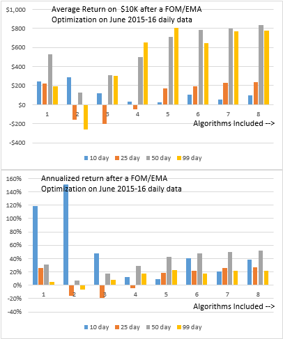
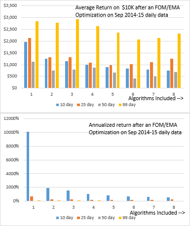
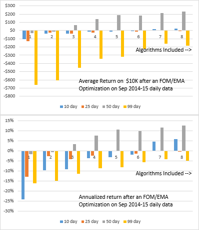
The top graph in each set shows the average return on $10K on running from one to 8 algorithms for a 10day, 25 day, 50 day or 90 day period on the out-of-sample data immediately following the 250 days of data the optimization were run on. So, for example, for the stock A (Agilent), the algorithms were found by using the data from June 15 2015 to June 9th 2016. The 10 day result was on the data from June 13th 2016 to June 24th 2016. The 25 day result was on data June 13th through July 18th 2016, and so on. These are trading days, not calendar days.

The buy-hold performance of this portfolio is shown below:

So if you had correctly guessed to go short for the 10 day period and long after that, you would have made more profit. On the other hand, if you had guessed wrongly, you would have been better off following the algorithms.


Percentage Band/Return optimization vs. EMA Band/Figure of Merit optimization

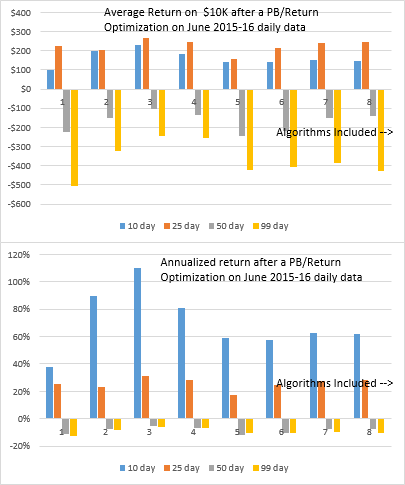
A three algorithm average for the PB/Return optimization for June 2015-16 gave the best Annualized Return (AR) results overall, much better than just running one algorithm. But there seems to be little point in running them beyond 10 days--profits barely increased for the next 15 days and by 50 days had soured into a loss.

The EMA/FOM algorithms had better longevity and, on average, were not lossy until after 50 days. Peak profits were at 25 days and slightly better than those for PB/Return, but best AR was still at 10 days, the same as the PB/Return result but in most cases lower.

The Figure of Merit optimizations gave more consistent results than simply optimizing for return, especially when averaged over several algorithms.

A-Z Portfolio Jan 2015-16 Optimizations

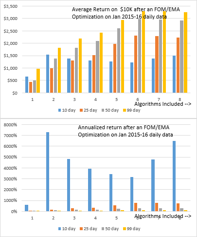
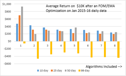
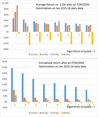
Again we see a breakdown in returns for the 99 day runs, but the shorter time-frame runs are all positive. Buy-hold performance for the same periods are shown below:

Running a single algorithm on each stock in the portfolio realized most of the potential profit for the 10 and 25 day periods, but running for 50 or 99 days gave disappointing results. Averaging across many algorithms did not lead to improvements.


A-Z Portfolio Sept 2014-15 Optimizations

Clearly, the best results for this timeframe were achieved when more algorithms were averaged, however the results were tepid at best and did not exploit the potential of the data, which is hinted at in the buy-hold performance for the portfolio in same time-frame, shown below:


Multi-algorithm trading strategy testing- Portfolio and Methodology

"Two heads are better than one", the saying goes. But can averaging improve trading systems? Can a multi-algorithm technique improve profitability and lower risk? After compiling the "Summary of Strategy Performance", I was very curious to quantify if and for how long strategies such as those published here were profitable for. To do that, I used out-of-sample testing which is very easy to do with SignalSolver.

In out-of-sample testing, you first find a strategy which worked for a specific time period. You then see how that strategy performed on data outside that specific time period. You can either go forward or backwards in time, but in these tests I go forward because that's pretty much how you would do it in reality. By multi-algorithm I mean running several algorithms simultaneously on the same stock. We look at running from 1 to 8 algorithms on each stock in a portfolio. Every stock has a different set of algorithms, found by optimization.

To get a handle on average success rates, I needed to analyze a reasonable number of stocks. Accordingly, I will report on 30 stocks with 128 out-of-sample results on each, a total of 960 algorithms each run for 4 time periods.

The A-Z Portfolio

I tried to create a portfolio which didn't look like I had cherry-picked stocks to put a rosy face on things. Accordingly, I used stock symbols A though Z which comprises 24 stocks (because symbols J and U are not assigned at this time). This I will call the "A-Z" portfolio. Other stocks were tested: AMZN, DUST, FAS, FB, NUGT, SPY and UWTI. I will report on these later, but the results are also in the spreadsheets if you are interested ahead of time. 

Methodology

I have been careful to ensure that anyone with a recent copy of SignalSolver can reproduce the results I report. You just need to make sure the Settings are as per the Settings tab on the results spreadsheets. Also, you will need to adjust the Web Query end date to get the exact OHLC data I used, (or increase the Offset to move the data back in time).

First, load the daily OHLC data for the stock into SignalSolver by typing the symbol and making sure data interval was set at "Daily". Set the "Days To Analyze" to 250 days which is almost a year of data and the Offset set to 100 days leading to an exclusion of the most recent 100 days. For example, for stock symbol "A" the included data was 6/15/15 to 6/9/16, the excluded data 6/10/16 to 10/31/16. Other exclusion days tested were 200 and 300 days. The buy and sell scan ranges were set to -20% to +20%, and the investment style set to "Long and Short", starting in the "Out" state. I'll talk about optimizations later.

Clear all the algorithms on the Algorithm tab (select the rows and press delete) so SignalSolver won't scan through any pre-configured strategies. Set the Seek/Scan level to "Seek level 2". and press Solve.  This will search 1000 algorithms using about 400,000 backtests. The seek doesn't search the same 1000 algorithms each time, but follows logic as to what may constitute a good strategy. It would take about 5 minutes to finish on my machine after which the top 100 algorithms will appear on the Algorithms tab, with the top 8 being transferred to the Strategy and Report Tabs.

For this study, I looked only at the top 8 strategies found. Here is an example Seek result:
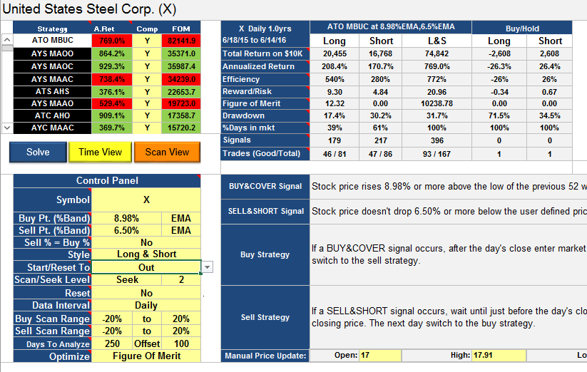
Example of a seek result

Example of a seek result

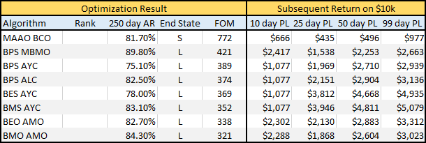
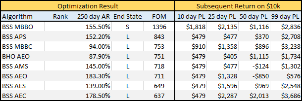
Notice that the strategies are ordered with the highest Figure of Merit first, as this was a FOM optimization (see below).

Next step is to see how each of these 8 strategies played out moving forward in time. I started out looking at the next 25, 50 days and 99 days, but it quickly became clear that I'd have to also look at a shorter time interval, so I opted for 10 days.

Start State of out-of-sample testing

Start State is the start state of the backtest and is especially important for the short time results as these may not trade much, if at all. I set the Start State of the out-of-sample test to Out, unless a clear Start State was indicated by the traffic lights on the 250/100 seek result. For example, in the above illustration, 5 algorithms are green (bullish) and 3 are red (bearish). Only if the vote was 6/2, 7/1 or 8/0 would I set the start state to that indicated by the traffic lights, Long for green and Short for red, otherwise use Out.

Reading of the out-of-sample result

After setting the Start State, I would read off the out-of-sample results by setting the "Days to Analyze" and the "Offset". Here is an example, same stock, same algorithms:
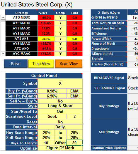
Out-of-sample result

Out-of-sample result

Notice the data analyzed starts from 6/16/16. I had to avoid using 6/15/16 data because it is used in the traffic light calculation, that's why I set the offset to 89 and not 90 days. Its vital that none of the backtested data is used in the out-of-sample analysis. After 10/89 I would set the Days To Analyze/Offset to 25/74, then 50/49 then 99/0. Each time I would cut and paste the top 8 Strategies and the Annual Returns into the results spreadsheet.

Optimizations and bands

I followed this procedure for two different Solve optimizations, one using a simple Return optimization on the Percentage Band (PB) (like most of the algorithms on this site), the other a Figure of Merit optimization using a 50 period (H+L)/2 Exponential Moving Average band. Why use an EMA band? It seemed to give better results than the PB band, but I haven't confirmed this properly yet.

Bands are explained here. The FOM optimization used these weights-
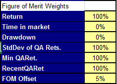
FOM Weights

With these FOM settings we are essentially looking for algorithms with good 250 day return, low standard deviation of returns for each quartus (62 days in this case), a good value for the minimum of all four quartus returns, and good returns for the most recent quartus. By setting up this kind of optimization we hope to avoid algorithms which performed very well for only short period. For more information on FOM, see here.

There is a secondary effect to running multiple algorithms on the same stock; a change in efficiency. All the tests were done using investment style "Long and Short", where you are essentially tying up the capital 100% of the time. If you run 2 algorithms  on the same stock, however, there may be times when algorithm A puts you long while algorithm B puts you short, effectively taking you (mostly) out of the market. Since, as I hope to show, profits on each algorithm average out to be similar, you have essentially increased the effective annual return by reducing the time your capital is in the market. We don't take this effect into account in the Annualized Returns reported here, we assume all capital is in the market for 100% of the time. But I believe this effect is real--please correct me if I am wrong about this.

In the next post, we shall look at the results.


IBB Trading Strategy Details and Performance

IBB Trading System (Weekly)

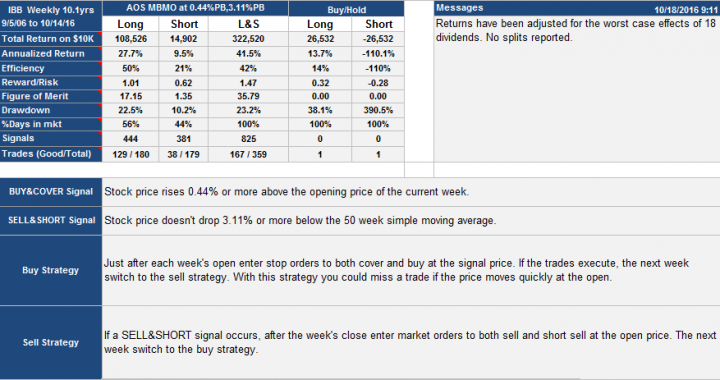
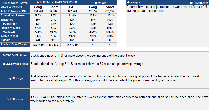
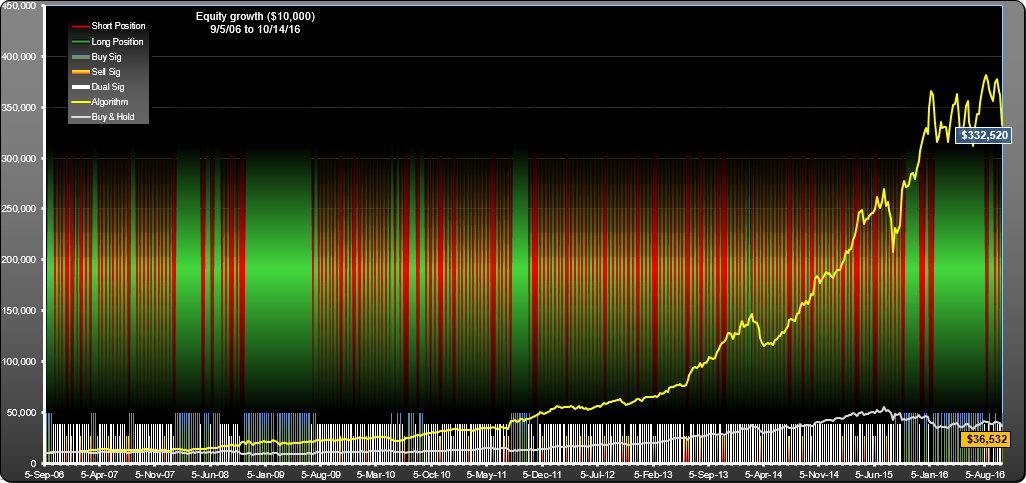
This weekly trading strategy for IBB had 3 times better annualized returns than IBB and more than 10 times better return over the 10.1 years. For each 2.5 year period within the 10 years,  the annualized return was between 30 and 50%.
IBB Trading Strategy Details and Performance

IBB Trading Strategy Details and Performance

IBB Weekly Trading Strategy: Equity Curve

IBB Weekly Trading Strategy: Equity Curve

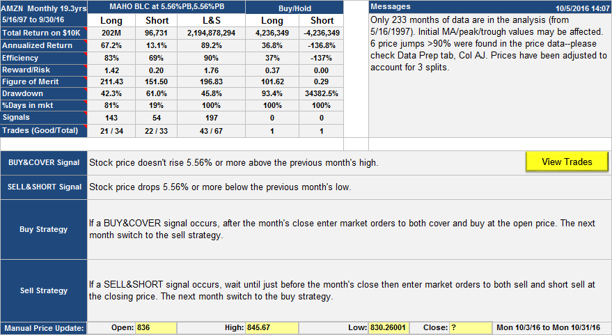
FEYE Trading System: Performance

FEYE Trading System

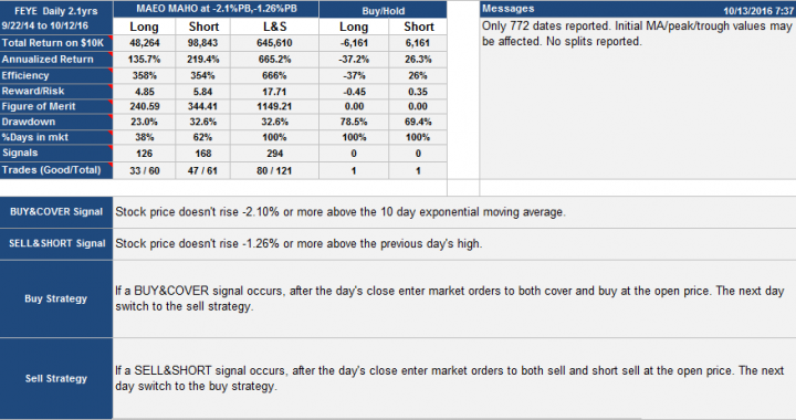
A trading system which worked for FEYE (FireEye). This is based on daily data, so traded at most once per day.

FEYE Trading System: Performance

FEYE Trading System: Performance

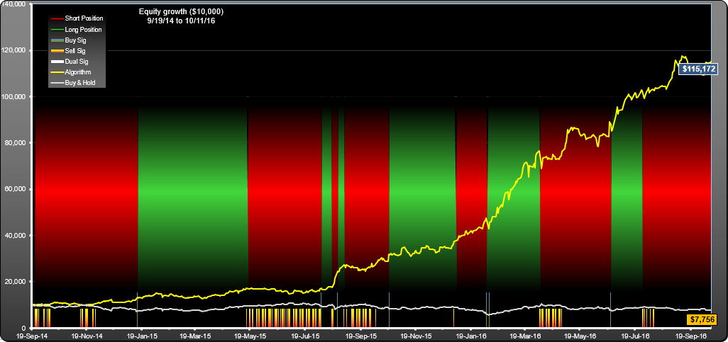
FEYE Trading System: Equity curve, signals and positions

FEYE Trading System: Equity curve, signals and positions

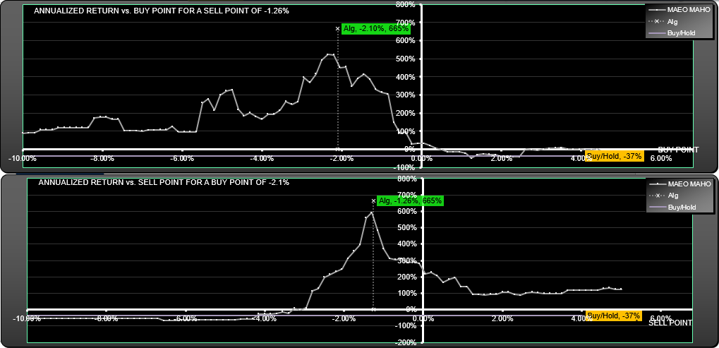
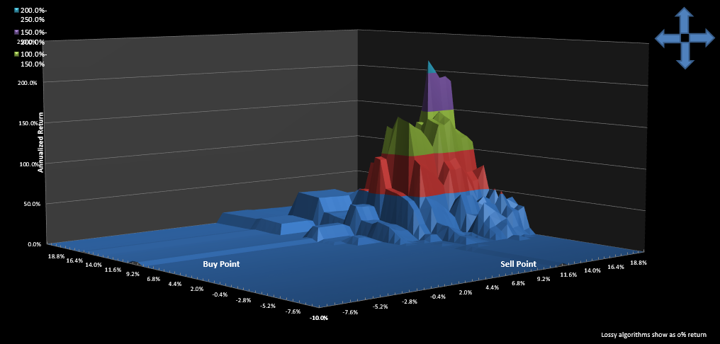
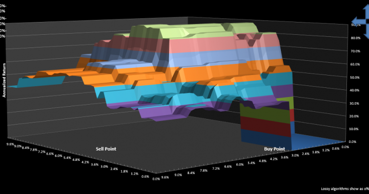
FEYE Trading System: Parameter surface

FEYE Trading System: Parameter surface

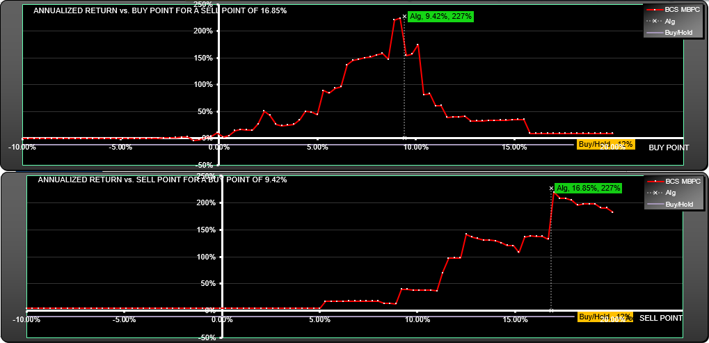
FEYE Trading System: Parameter scan

FEYE Trading System: Parameter scan

FEYE Trading System: Trades List

As always, future performance is not guaranteed.

AMZN 20,000,000% total return

Over 500 times better return than buy-hold

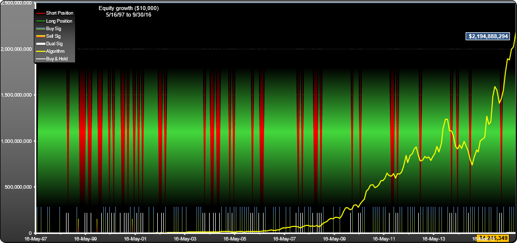
In the time frame May 16th 1997 to Aug 1st 2016, this strategy gave a return of 88.9% compounded which amounts to over $219,000 for every dollar invested, that's 518 times better than the performance of buy-hold which only gave $423.

This screenshot shows the strategy description and performance along with messages warning if something looks odd about the data. The data was checked and all the price jumps turn out to be real with the prices agreeing with prices from other sources.

amzn-m-table

The strategy used Long and Short investment style, so was always in the market long or short. The short side trades didn't do nearly as well as the long side trades, but well enough to boost the overall performance by a factor of almost 10. Also, the short trades had an efficiency of 69%, so for the short time that the strategy was short it did quite well.

Trading was at most once per month, trading a total of 67 round trips over the lifetime. 43 of these trades were good

This is a straightforward type of Percentage Band algorithm. Buy signals occurred in months when the stock price failed to rise, at any time, 5.6%  above the high of the previous month. This happened 143 times out of the 243 months of data. The buy was at the following month's open, but it only happened 34 times because the position was already long in most cases.

Sell signals occurred whenever the stock price fell 5.56% below the previous month's low at any time in the month. Usually, there was a buy signal the same month as a sell signal; there were 92 buy signal only months, 3 sell signal only months and 53 dual signal months. For this type of algorithm, if you are long you have to sell if a sell signal occurs, and you have to buy if a buy signal occurs when you are short. This is all explained in this video.

Here is the equity curve for the strategy, along with the signals and positions mapped out.

amzn-m-equity-curve

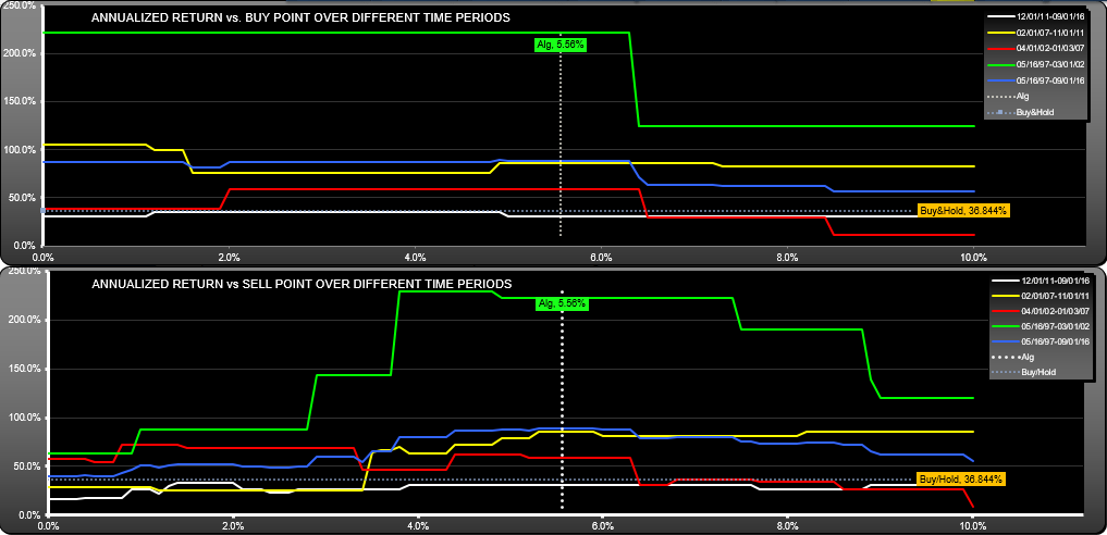
It looks as though the equity curve is still rising rapidly, however a closer look at the returns over different time periods (below) shows that most of the strategy gains occurred in the 1997 to 2002 time period. In fact, in the most recent quartus  (one fourth of the data, 2011 -16) the strategy did not quite keep up with buy/hold (31% vs 35.6% annualized).

amzn-m-longevity-scan

amzn-m-longevity

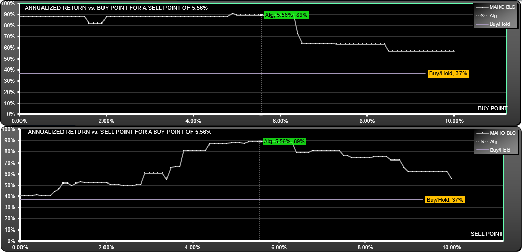
Looking at how changes in the parameters affect return, we see a broad area over which the buy parameters worked with a slightly narrower range for the sell parameter.

amzn-m-return-scan

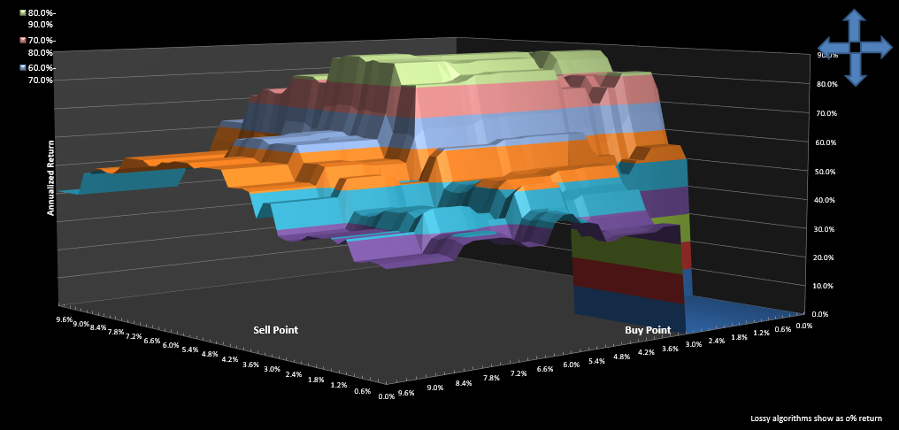
The parameter surface shows a nice large structure, showing that sensitivity to parameter changes was fairly low, but remember most of the gains were focused in the 97-02 timeframe.

amzn-m-return-surface-scan

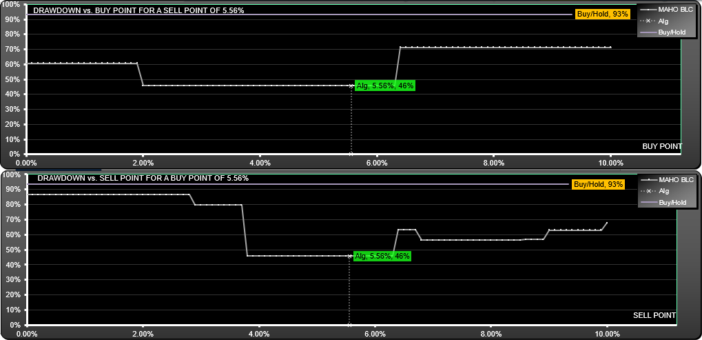
Drawdown for the strategy was much better than for buy-hold (46% vs 93%) and not overly sensitive to parameter change:

amzn-m-drawdown-scan

You can take a look at the buy-sell points on the trades list. As always, please be aware that there is no guarantee that this strategy will work in the future.

Recent performance

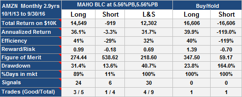
For the most recent 2.9 years, here is the performance table.

amzn-m-recent-table

There are not enough trades to make any firm conclusions about where the optimum parameters are now, but there is evidence to suggest that the buy point has pulled in somewhat. I suggest you download SignalSolver and optimize for different timeframes to get a feel for where the parameters might have moved to.