The SignalSolver Help System
The Stock Symbol dialog is located on the Wizard Tab after clicking "Click to Start SignalSolver"
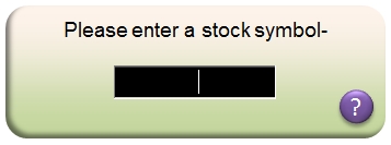
Entering a Stock Symbol
You can enter any stock symbol recognized by Yahoo Finance, the spreadsheet will then fetch all the historic price data needed for analysis. If the symbol is not listed on the NYSE, NASDAQ or AMEX exchanges, you should follow the symbol with a dot, then the exchange code.
Examples of valid symbols would be:
F Ford Motor Company (NYSE)
TSCO.L Tesco (PLC)--London Stock Exchance
R.TO Romarco Minerals (Toronto Stock Exchange)
2330.TW Taiwan Semiconductor Manufacturing (Taiwan Exchange)
^RUT Russell 2000 Index
XSIIX Ing Senior Income I (Mutual Fund)
If you enter a mutual fund symbol, remember that mutual fund prices only change once a day, which can limit the algorithms available to you depending on the data interval chosen.
SignalSolver fetches several tables, the historic price data, split/dividend data, spin-off information and backup split information if necessary. It can take a few seconds. This is the only interaction SignalSolver has with external sites, except for these links to the help pages. Once the data is loaded it is checked for certain errors and any corrections are flagged and you can check it by looking at the DataPrep, Strategy or Analysis tab.

The Control Panel is situated on the Report tab
The Control Panel
The Control Panel is situated on the "Report" tab. It is used to change the major parameters affecting the program.
Symbol
Enter a stock symbol as described above. Entering a stock symbol in the control panel will trigger a price fetch for the symbol, but it won't start the solver.
Buy Point and Sell Point
Buy and sell points are signal trigger points a fixed percentage (for PB--percentage band) or a percentage of the selected band above or below the reference price. The band is selected immediately to the right of the percentage value. When the price hits the buy or sell point a signal will occur and a transaction may follow depending on the position currently held. You can manually set the buy and sell points by entering percentages in these boxes. You can also change this value by clicking on a point in a scan graph. SignalSolver scans though a hundred buy-sell points and graphs the results for each of eight algorithms..
Sell % = Buy %
If you set "Sell % = Buy %" to "Yes", the sell point is forced to be equal to the buy point for Solving. You may wish to do this if you are looking for symmetrical algorithms where the buy and sell points are the same. Solving is much faster if this is set to "Yes", but the algorithms found are often not as interesting.
Style
The three investment styles are "Long", "Short" and "Long & Short". In the L&S investment style you are always in the market, either long or short. The style is selected in this box.
Start/Reset to
You specify here how you wish the algorithms to start out on day one, either "long", "short" or "out". If you have specified a Reset (see below) at the close or open, the algorithm will always reset to the state specified at the close or open.
Scan/Seek Level
Select either "Scan" or "Seek" and a level from 1 to 9. In "Scan" mode the solver will only scan the algorithms on the algorithm tab, and only those with a scan level less or equal to the Scan Level. You can add and remove algorithms as you see fit to the algorithm tab and set the scan level appropriately.
In "Seek" mode, the solver will first scan through all the algorithms on the Algorithm tab which have a non-zero scan level. It will then search for strategies outside of the scan space using a search based on buy and sell signals it considers likely to succeed. In this context, the level is related to the number of algorithms to be examined. For example level 1 will search up to 500 additional strategies, level 8 will search up to 40,000. Seek Level 9 will always search the entire strategy space up to 186,000 strategies depending on which strategies are set up in the Seek Inclusions. This can take 24 hours or more.
Reset
You can set up the algorithms so they reset either at every open or close the value set up in the "Start/Reset to" cell above. Applying a reset means that the algorithm will start each day in the same state, "Long", "Short" or "Out" i.e. out of the market.
Data Interval
Choose Daily, Weekly or Monthly data. Each time interval will have one Open, High, Low, Close data point. Trading strategies will be based on the data interval, at most there will be one round trip trading cycle per data interval.
Buy-point and Sell-point Range
When scanning the algorithms, the buy-point and sell point values are constrained by the range entered here. The same range will appear on the x axis of each of the Scan View graphs. Ranges can include negative numbers.
Days/Weeks/Months to Analyze
Determines how many days/weeks/months to include in the testing. Can be in the range 2 to 528. Note there are typically 252 trading days a year. "Offset" allows you to exclude the specified number of recent days/weeks/months from the analysis. For example, if Offset were set to 100, the most recent 100 days/weeks/months would be excluded from the analysis. After finding an algorithm you could then set the Offset to zero to see how the algorithm fared on the most recent data. This is sometimes called out-of-sample testing. Setting the Offset does not change the number of days analyzed, it shifts the analysis range back in time, but remember, there are only 800 points total available, and if you move backwards that far, the moving averages, peaks and troughs will be inaccurate. An alternative is to change the webquery dates on the Settings tab.
Optimize
Determines what the solver optimizes for when searching for the best strategies. Can be-
- Return
- Efficiency
- Risk-Reward
- Figure of Merit
The Strategy Selection pane is located on the Report tab
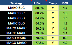
The Strategy Selection Pane
We give unique names to trading strategies by using acronyms which fully describe the way the strategy works. In the Strategy panel you will see the acronyms of eight algorithms which can be selected for viewing and comparing. Click on the acronym to view the strategy. If there are more than 8 results in the Algorithm Table, you will see the scroll bar appear next to the Strategy Table which allows you to scroll through all the results. The colors of the second and fourth columns indicate algorithm disposition for the last day, week or month of the analysis--bullish (green) or bearish (red). A yellow entry indicates that the strategy died at some point by exceeding the maximum allowed drawdown.
Comparing Algorithms
The Comp column shows if an algorithm is included on the Comparison graphs. Double click on the Comp "Y" or "N" to toggle the strategy into or out of the comparison. Comparisons are activated by clicking on the "Compare" button in the Scan View.
The A.Ret Column
The annualized return of each strategy.
The Eff-R/R-FOM Column
The final column changes depending on the Optimization strategy selected: Efficiency, Risk-Reward or Figure of Merit.
The Performance Table is located on the Report tab
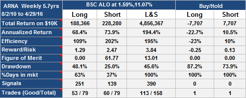
The Performance Table
We show the performance for the Long and Short side of the algorithm. Long will show the performance if you had just bought and sold and never went short. Short shows the performance if you had only sold short and covered and never gone long. The third column shows the overall performance for the selected Style, in this case Long & Short, in which you are always either long or short. The last two columns show Buy and Hold performance for both Long and Short.
Total Return
The compounded return for the strategy on a $10,000 investment, that is the return if all profits had been re-invested. It is measured over the period of the algorithm (in the Days to Analyze control) so is not annualized. In the example shown, the L&S return is much higher than the individual Long or Short return for the algorithms. This is because the combined compounded return will be (1+Long Ret)*(1+Short Ret)-1. If you wish to know the simple returns, please refer to the Analysis tab. Trading costs are included if a commission and/or slippage is entered. The initial amount ($10,000 is the default) can also be changed on the Strategy tab.
Annualized Returns
The annual compounded return for the strategy, This assumes all profits are re-invested. Commissions and slippages are included if set on the Strategy tab.
Efficiency
The compounded return divided by the %days in mkt. It represents the hypothetical return if you could have invested with the same rate of return for 100% of the time. (Note that compounding would increase this hypothetical return even higher).
Reward/Risk
The compounded return divided by the sum of the drawdown and the drawdown offset . Higher is better. The drawdown offset a user configurable percentage which can be used to prevent the reward/risk from going to infinity on zero drawdown strategies.
Figure of Merit
An indication of the relative merit of an algorithm, but not to be taken too seriously. Figure Of Merit (FOM) goes up with return, but down as Time in Mkt and Drawdown increase. You can control the amount of influence each of these factors has, see FOM Weightings below. Higher is better.
Drawdown
The greatest loss you could have incurred had you bought on a peak and sold on a subsequent trough. We use drawdown as a measure of risk. Lower is better.
%Days in Mkt
The percentage of days where a position was held. If a position was held for a partial day, it is counted as one full day, unless both a long and short position was held on a particular day, in which case 0.5 days is assigned to each. Refer to the Analysis tab in the "Days in Mkt" column to understand how this figure was arrived at. The figure is an approximation and tends to be higher than the actual percentage of time positions were held. You can optionally switch to showing "%Time in mkt" instead of "%Days in mkt", see Days or Time below.
Signals
The number of buy (long) and sell (short) signals. Not every signal leads to a trade, for example if a buy signal comes along and the algorithm is already long, then no buy will occur.
Trades (Good/Total)
The number of profitable round trip trades/the total number of round trip trades. Each long trade is one buy and one sell. Each short trade is one short sell and one cover. A single reversal, long to short or short to long counts as one round trip trade.

The Signals and Strategies Table is situated on the Report tab during Table View
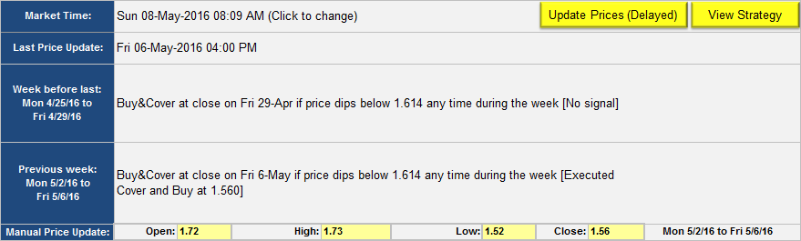
The Signals and Strategy Descriptions Table
The Signals and Strategy Descriptions Table on the Report tab gives detailed information on the selected trading strategy. It is visible whenever Table View is selected.
Buy and Sell Signals
Gives a description of the buy and sell signals.
Buy and Sell Strategies
Describes both the buy and sell strategies.
View Trades Button
Switches to the Trades view, which shows trading activity for the last two trading periods of the analysis.
Update Prices (Delayed) Button
Updates the current stock prices from the web. Prices are typically delayed at least 15 minutes by the information provider.
Manual Price Update
Allows you to enter up-to-date price information manually, which in turn updates the Trades information.
Backtest Tables appear both on the Strategy and Analysis tabs
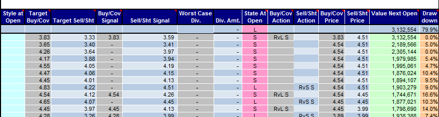
The Backtest Tables
Backtest tables give you a detailed view into what happened on each time period of the simulations.
Style at Open
This column shows the style, which in this edition is the same at every open; L (long), S (short) or Blank (Long and Short)
Target Buy/Cov and Sell/Sht
The target prices are shown here. If these targets are hit a signal is generated. You can also set up the algorithm to generate a signal if a target is missed. Targets are re-calculated every time period, for example for a daily algorithm, targets are calculated daily .
Buy/Cov and Sell/Sht Signals
Signals are generated when the Target prices are hit (or sometimes if they are missed). However price shown here will be the transaction price, which is usually the same as the Target price if the transaction time is set to Signal, but not always. If the Open price meets the target criteria, the signal will reflect the Open price. Not all signals lead to a buy/cover or sell/short action--for instance,the buy signal can't be acted on if the position is already long.
Dividend per Stock
Dividends can have a significant influence on performance for large cap monthly based strategies. This column reflects any dividend amount reported during the period, per stock.
Div Amt (Worst Case Div. Amt)
The dividend amount paid or owed, worst case. If you owned the stock for the whole period in which the dividend was paid, you will receive the dividend. If you were short for the whole period, you will owe the dividend. If there were transactions during the period it's not always possible to determine if the dividend amount was positive, negative or zero because there is not enough price-time data to determine the exact time of the transaction in relation to the dividend payment. SignalSolver assumes the worst, so you can be sure that the total dividend amounts are equal or lower than actual dividend amounts would have been.
State at Open
This column shows the the position just after the open as Long (L), Short (S) or no position (Blank). If there was a transaction at the open, this reflects the position just after the transaction, for example if there was a sell at the open, this will show no position (Blank).
Buy/Cover and Sell/Short Action
When signals lead to transactions, there will be an entry in this column. The entry indicate the type and the source of the transaction. Transaction types are--
- Buy (open a long position)
- Cov (close a short position)
- Sell, (close a long position)
- Sht, (open a short position)
- RvL, (reverse long--close a short and open a long position at the same time)
- RvS, (reverse short--close a long position and open a short position at the same time)
- C/B, (cover or buy, depending in what order signals arrive)
- S/Sh, (sell or short, depending on signal order)
The suffix refers to the source of the transaction
- S results from an "at signal" target strike
- C results from a target strike with a transaction time of at Close
- O results from a target strike with a transaction time of at Open
- c results from a reset at the close
- o results from a reset at the openl
- H a hypothetical transaction
hypothetical transactions can arise in a number of ways. See here for more details.
Value Next Open
Value of the position or cash at the next open. All returns are compounded, that is all profits and losses are reinvested in the algorithm. To see simple return, spotlight the algorithm you are interested in and check the Analysis tab under Simple Return. No trading overhead costs are included in any of the returns calculations.
Drawdown
We define drawdown as the maximum percentage decline over the life of the algorithm. Measured from a peak to a trough, its effectively the most you could have lost if you had invested in the algorithm for one random period of time. We use it as a measure of risk in the reward/risk calculations.

Analysis Tab Fields
The Analysis tab copies the algorithm spotilighted in the Control Panel from the Strategy tab for more detailed analysis and graphing. We do the analysis for both the Long and Short sides of the algorithm.
Algorithm Long/Algorithm Short
In these columns we show the return and drawdown for the long and short side of the algorithm. The results are displayed in the performance table and on the Growth Graph on the Results tab.
Days in mkt
If a position was held for a partial day, it is counted as one full day, unless both a long and short position was held on a particular day, in which case 0.5 days is assigned to each. This can lead to different percentages for "Days in mkt" if you switch between SAR and Long/Short styles. The figure is an approximation and tends to total higher than the actual time positions were held.
Time in mkt.
Time in mkt is a estimate of the actual time that Long and Short positions are held for. It will total less than the "Days in mkt" figure above because partial days are only assigned a fraction of a day, not a whole day. If a buy or sell occurs, it counts as Long for a half day. If a short sell or cover occurs it counts as Short for half a day. If a C/B and S/Sh cycle occurs, since we don't know if a buy/sell cycle or a cover/short cycle was executed (it depends on signal arrival order), we assign one quarter day to each Long and Short.
Optionally, you can display Time in mkt in the performance table and use it in the FOM and efficiency calculations, but the buy/sell point scans will always display Days in mkt.
Sliding Returns
The compounded return for the last N trading days, where N is the number at the top of the column and can be set by the user. This data is used in the longievity graph.
Profit and Loss
We generally use compounded returns in all the analyses, where profits/losses are re-invested. If you are interested in simple returns, they are shown here. The simple return would be the profit/loss realized if you always invested the exact same amount of cash for every transaction. Typically simple returns produce less profit and more loss than compounded returns (in fact simple losses can exceed 100%, compounded losses can't). As with compounded returns, transaction fees are not included. There are three columns because occasionally you will run into the situation where a profit or loss cannot be attributed to Long or Short position. Specifically, if reset is active and the reset state is Out, then a C/B and S/Sh cycle can occur. However whether the algorithm went long or short will depend on the order of arrival of the signals. On these days you will see "C/B" in the "Buy/Cov Action" column and "S/Sh" in the "Sell/Sht Action" column.
At the bottom of the column you will also see how many of the trades were good (i.e profitable) and how many were bad. Also, we give the average P/L per trade--the simple return divided by the number of postions held.

Settings Tab--General Settings
Settings Tab-GeneralSettings
These settings are located on the left side of the Settings tab.
Amount
Sets the starting amount for the simulations. Default is $10,000.
Commissions and Slippage
We allow for a fixed cost per trade commission, and a fixed percentage per trade slippage value. Slippage is sometimes used to account for bid-ask spreads, but you need to think about setting the value carefully for each strategy since they can use limit orders.
Weeks in Peak and Trough
Sets the number of weeks used on daily and weekly data for the peak and trough (P and T references). Default is 52 for both.
Months in Peak and Trough
Sets the number of months used on monthly data for the peak and trough (P and T references). Default is 12.
Use Div Adjusted Prices
Allows the program to use the dividend adjusted prices instead of split/spin-off adjusted prices. When running SignalSolver simulations, we recommend NOT to use dividend adjusted prices for two reasons; Firstly, dividend adjusted data gives incorrect prices for any historic price point prior to a dividend. If a dividend is paid today, and you adjust backwards, yesterdays adjusted prices no longer reflect actual prices, so moving averages, peaks, troughs and even open, highs, lows and closing prices are all wrong. Secondly, if you are using weekly or monthly prices and a dividend occurs during a month, you don't know how to adjust the high and low of that week/month because you don't have enough data to know if the dividend occurred before or after the high or low. For these reasons and others, we prefer you use split adjusted prices (set this field to NO) and let the program add in the worst case dividend effects mathematically using actual dividend data.
If using dividend adjusted prices, all worst-case dividend calculations are turned off and you will see all zeros in the dividend columns.
Days or Time
Switches between %Days or %Time display. See Analysis field settings above. This field determines what is displayed in the performance table, however the FOM optimizer and buy/sell point scans will always use %Days in mkt.
Drawdown Exit
You can set this to a percentage value. The backtest is halted if the drawdown percentage exceeds this number, and the strategy is tagged with a yellow sentiment entry in the Strategy Selection tab. Default is 100%.
Speech Alerts
For long seeks and scans, SignalSolver provides a speech alert when the solver has finished its work. You can turn this feature off here.
Signals at Close only
Normally, SignalSolver looks at the high and low of each period (day, week or month) to determine if a buy and/or sell signal was generated. If this flag is set to "Yes", high and low prices are not used, only the close price of the period is used to determine if a buy or sell signal was generated.
Web Query Start and End Dates
The end date is set to "=TODAY" by default, but can be changed here.The start date is formula based to cover the 528 data periods plus any SMA, EMA, peak or trough data required. 4 years (daily), 16 years (weekly), 65 years (monthly).
Price Jump Threshold
We flag price jumps in the price data within a period so that the user can check for split or spin-off information which is occasionally missing from the webqueries. The price jump message will appear in the messages space of the Reports tab and also in the Yellow messages dialog of the Wizard tab. The ratios we look at are Open/Close, Close/Open, High/Open, Open/Low and High/Low. If any of these exceed the threshold, a flag is raised. When price jump thresholds are exceeded, it does not necessarily mean the prices are bad, just that they should be checked (on the Data Prep Tab).
SMA Periods
The simple moving average for N periods is computed by adding together the previous N closing prices and dividing by N. When using SMAs, a price anomaly has the same impact for N days, then it suddenly goes to zero.
SMA Prices
The simple moving average price can optionally be calculated from the Closing Prices (C), the Median Prices (H+L)/2, the Typical Prices (H+L+C)/3 or the Weighted Closing Prices (H+L+2C)/4.
EMA Periods.
This number is used in calculating the Exponential Moving Average reference prices. The EMA is computed using the previous closing prices. The moving average is computed from
NewAverage= (ClosingPrice + (M-1)*OldAverage)/M , where M=(EMAPeriods+1)/2
When using an EMA, the influence of a price anomaly gradually diminishes.
EMA Prices
The expoonential moving average price can optionally be calculated from the Closing Prices (C), the Median Prices (H+L)/2, the Typical Prices (H+L+C)/3 or the Weighted Closing Prices (H+L+2C)/4.
Settings Tab-Scanning Settings
These settings are located in the central area of the Settings Tab.
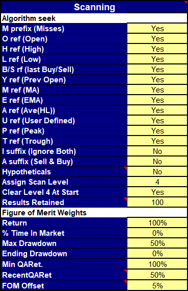
Algorithm Seek Settings
Seek Inclusions
Controls which strategies are included in the Seek. We don't normally recommend you include hypotheticals as these strategies require a time machine to implement. However, these may be interesting. They tend to dominate the Seek results and you can attempt to emulate them in your trading, When using Sentiment you may not care that hypothetical algorithms cannot be implemented.
Assign Scan Level
The results of the Seek are assigned a scan level which you can view on the Algorithms tab. The standard setting is 4.
Clear Level <N> at Start
You will normally clear out the results of a previous Seek at the start of the new seek by setting this to "Yes", If set to "No" the old Seek results will not be cleared at the start of the new Seek.
Results retained
The solver can test tens of thousands of algorithms. It saves the best N results and writes them to the Algorithm Table on the Algorithm tab. You scroll through them using the scroll bar on the Strategy Table. Default is 100.
Figure of Merit Weightings
The Figure of Merit (FOM) is a number assigned to each backtest result which SignalSolver uses to compare in the optimization process if you set Optimize to FOM. It is arrived at by combining several parameters from the backtest result-
- Total return
- % Time in market (inversely related)
- Max Drawdown: the worst drawdown for the Days to Analyze period (inversely related)
- Ending Drawdown: the drawdown at the end of the Days to Analyze period (inversely related
- Minimum QA return (Rewards algorithms which didn't do badly in any quartus)
- Recent QA return (Rewards algorithms which did best in the most recent quartus)
A quartus is simply one fourth of the data. If the weight of an parameter is set to zero, then that parameter does not figure into the FOM. As you increase the weight from 0 to 100%, the parameter factors in more. Mathematically, we raise each parameter to the power of the weight then either multiply or divide by that factor. The FOM Offset is first added to all the inversely related parameters to prevent division by zero.
The standard deviation of quartus returns allows you to look for the most consistent returns quartus to quartus, but using it will penalize algorithms which performed particularly well or badly in one quartus. Minimum quartus return allows you to find algorithms which performed well across every quartus, even though they may not be consistent.
The numeric value of the FOM has no meaning other than to compare the performance of different strategies.

Settings Tab-Band Settings
These additional settings are located on the Strategy Tab.
Algorithm Band Setting
How bands work
This video gives a general overview of bands and how they work:
Periods
The number of OHLC periods to include in the creation of the band.
Scaler
Each band can be scaled up or down so that the buy and sell points are in a compatible range for all the bands. This avoids having to change the scan range as the band is changed. For example, if the scaler was 10 and the buy point was 20%, this would correspond to 200% or 2x the band.
BOL1 and BOL2 Settings
BOL1 and BOL2 are Bollinger series, created by taking the standard deviation of the prices in the previous period. The data series used in the SD calculation can be set to be the closing prices, the Median Prices (H+L)/2, the Typical Price (H+L+C)/3 or the Weighted Close Price (H+L+2C)/4. Default is the Median Price. Bollinger Bands are usually used in conjunction with a moving average reference such as SMA (M reference) or EMA (E reference)
KEL
A Keltner channel is a series made up of an exponential moving average of either the True Range or the High minus the Low of each OHLC period. Often used in conjunction with the SMA (M reference) or EMA (E reference).
RSI
The RSI band is the price differential from the previous closing price that would be required to meet the RSI Value Setting. For example, if the Value setting is 70.0, the band would give the price movement required to achieve an RSI of 70%.
TMTR
A trimmed mean of the True Range. It uses the mean taken by excluding a percentage of data points (set by the Value parameter) from the top and bottom tails of the data set.