"Two heads are better than one", the saying goes. But can averaging improve trading systems? Can a multi-algorithm technique improve profitability and lower risk? After compiling the "Summary of Strategy Performance", I was very curious to quantify if and for how long strategies such as those published here were profitable for. To do that, I used out-of-sample testing which is very easy to do with SignalSolver.
In out-of-sample testing, you first find a strategy which worked for a specific time period. You then see how that strategy performed on data outside that specific time period. You can either go forward or backwards in time, but in these tests I go forward because that's pretty much how you would do it in reality. By multi-algorithm I mean running several algorithms simultaneously on the same stock. We look at running from 1 to 8 algorithms on each stock in a portfolio. Every stock has a different set of algorithms, found by optimization.
To get a handle on average success rates, I needed to analyze a reasonable number of stocks. Accordingly, I will report on 30 stocks with 128 out-of-sample results on each, a total of 960 algorithms each run for 4 time periods.
The A-Z Portfolio
I tried to create a portfolio which didn't look like I had cherry-picked stocks to put a rosy face on things. Accordingly, I used stock symbols A though Z which comprises 24 stocks (because symbols J and U are not assigned at this time). This I will call the "A-Z" portfolio. Other stocks were tested: AMZN, DUST, FAS, FB, NUGT, SPY and UWTI. I will report on these later, but the results are also in the spreadsheets if you are interested ahead of time.
Methodology
I have been careful to ensure that anyone with a recent copy of SignalSolver can reproduce the results I report. You just need to make sure the Settings are as per the Settings tab on the results spreadsheets. Also, you will need to adjust the Web Query end date to get the exact OHLC data I used, (or increase the Offset to move the data back in time).
First, load the daily OHLC data for the stock into SignalSolver by typing the symbol and making sure data interval was set at "Daily". Set the "Days To Analyze" to 250 days which is almost a year of data and the Offset set to 100 days leading to an exclusion of the most recent 100 days. For example, for stock symbol "A" the included data was 6/15/15 to 6/9/16, the excluded data 6/10/16 to 10/31/16. Other exclusion days tested were 200 and 300 days. The buy and sell scan ranges were set to -20% to +20%, and the investment style set to "Long and Short", starting in the "Out" state. I'll talk about optimizations later.
Clear all the algorithms on the Algorithm tab (select the rows and press delete) so SignalSolver won't scan through any pre-configured strategies. Set the Seek/Scan level to "Seek level 2". and press Solve. This will search 1000 algorithms using about 400,000 backtests. The seek doesn't search the same 1000 algorithms each time, but follows logic as to what may constitute a good strategy. It would take about 5 minutes to finish on my machine after which the top 100 algorithms will appear on the Algorithms tab, with the top 8 being transferred to the Strategy and Report Tabs.
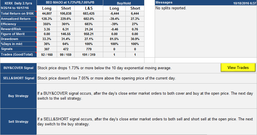
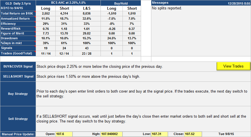
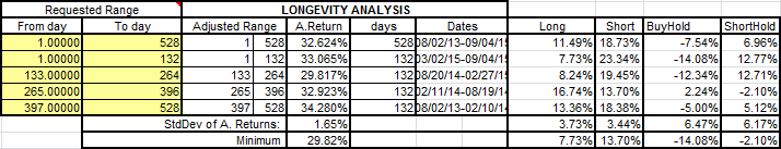
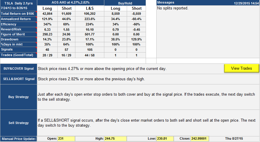
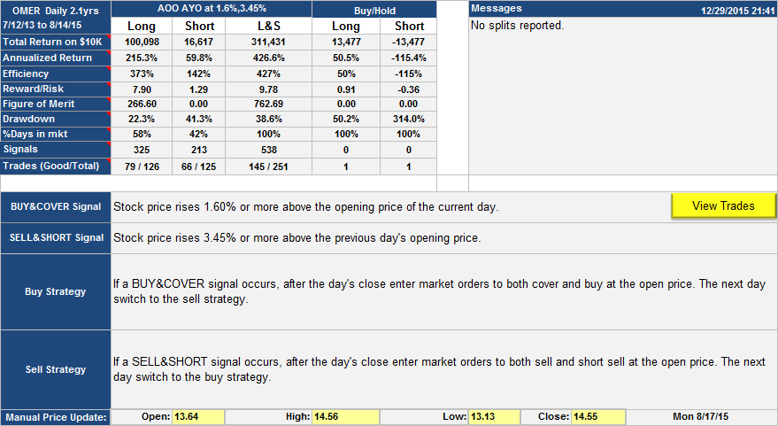
For this study, I looked only at the top 8 strategies found. Here is an example Seek result:
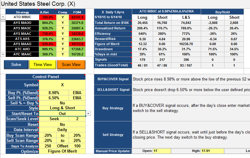
Example of a seek result
Notice that the strategies are ordered with the highest Figure of Merit first, as this was a FOM optimization (see below).
Next step is to see how each of these 8 strategies played out moving forward in time. I started out looking at the next 25, 50 days and 99 days, but it quickly became clear that I'd have to also look at a shorter time interval, so I opted for 10 days.
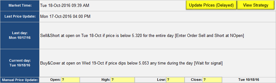
Start State of out-of-sample testing
Start State is the start state of the backtest and is especially important for the short time results as these may not trade much, if at all. I set the Start State of the out-of-sample test to Out, unless a clear Start State was indicated by the traffic lights on the 250/100 seek result. For example, in the above illustration, 5 algorithms are green (bullish) and 3 are red (bearish). Only if the vote was 6/2, 7/1 or 8/0 would I set the start state to that indicated by the traffic lights, Long for green and Short for red, otherwise use Out.
Reading of the out-of-sample result
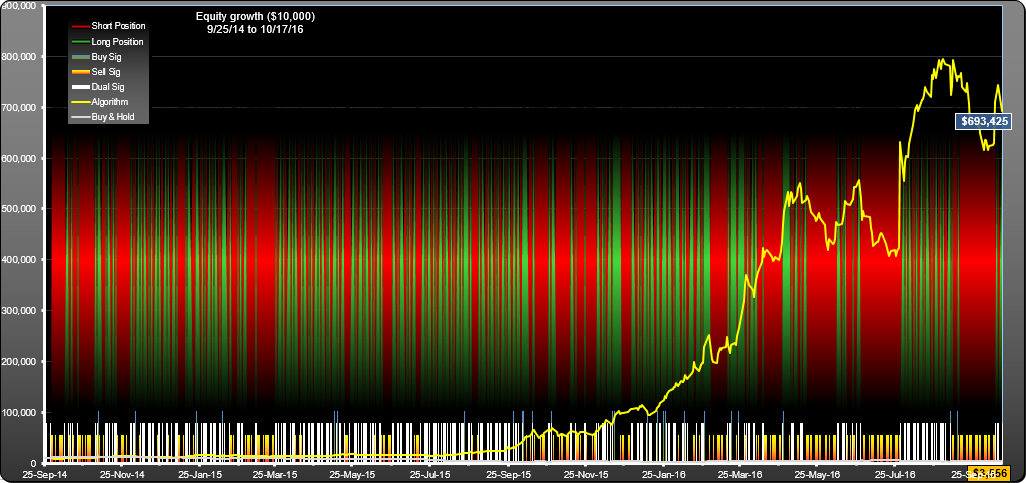
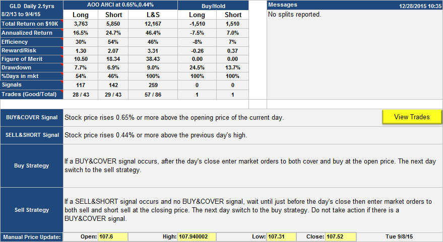
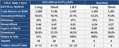
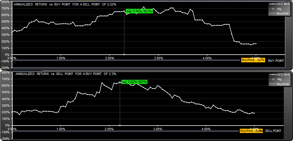
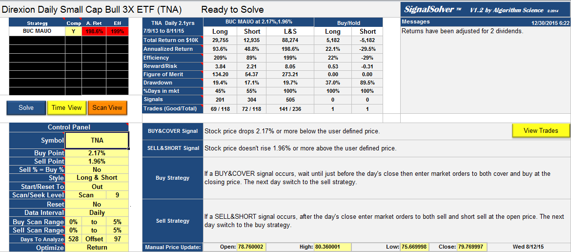
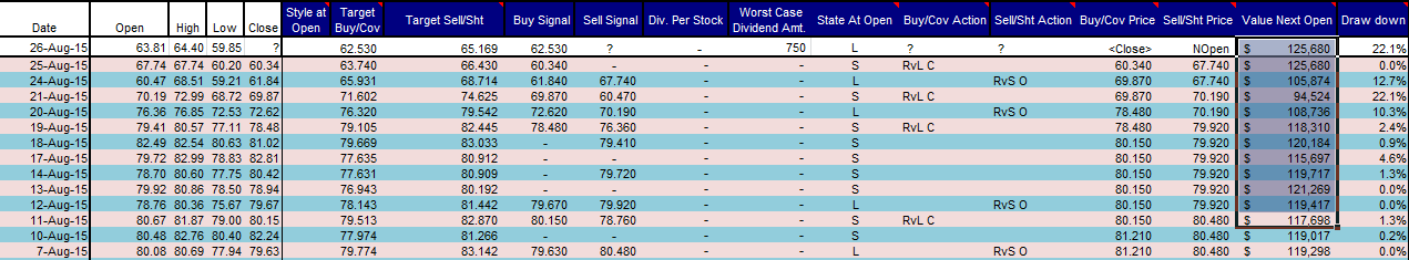
After setting the Start State, I would read off the out-of-sample results by setting the "Days to Analyze" and the "Offset". Here is an example, same stock, same algorithms:
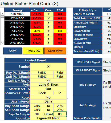
Out-of-sample result
Notice the data analyzed starts from 6/16/16. I had to avoid using 6/15/16 data because it is used in the traffic light calculation, that's why I set the offset to 89 and not 90 days. Its vital that none of the backtested data is used in the out-of-sample analysis. After 10/89 I would set the Days To Analyze/Offset to 25/74, then 50/49 then 99/0. Each time I would cut and paste the top 8 Strategies and the Annual Returns into the results spreadsheet.
Optimizations and bands
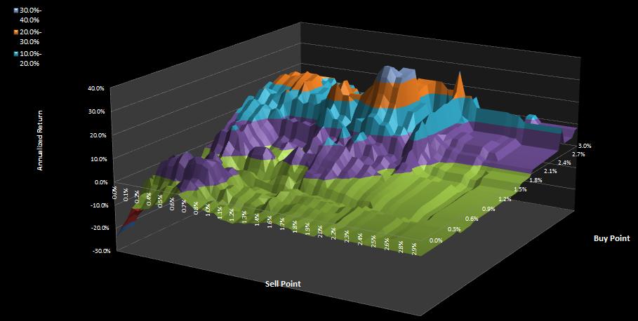
I followed this procedure for two different Solve optimizations, one using a simple Return optimization on the Percentage Band (PB) (like most of the algorithms on this site), the other a Figure of Merit optimization using a 50 period (H+L)/2 Exponential Moving Average band. Why use an EMA band? It seemed to give better results than the PB band, but I haven't confirmed this properly yet.
Bands are explained here. The FOM optimization used these weights-
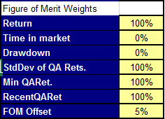
With these FOM settings we are essentially looking for algorithms with good 250 day return, low standard deviation of returns for each quartus (62 days in this case), a good value for the minimum of all four quartus returns, and good returns for the most recent quartus. By setting up this kind of optimization we hope to avoid algorithms which performed very well for only short period. For more information on FOM, see here.
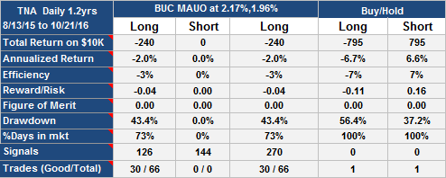
There is a secondary effect to running multiple algorithms on the same stock; a change in efficiency. All the tests were done using investment style "Long and Short", where you are essentially tying up the capital 100% of the time. If you run 2 algorithms on the same stock, however, there may be times when algorithm A puts you long while algorithm B puts you short, effectively taking you (mostly) out of the market. Since, as I hope to show, profits on each algorithm average out to be similar, you have essentially increased the effective annual return by reducing the time your capital is in the market. We don't take this effect into account in the Annualized Returns reported here, we assume all capital is in the market for 100% of the time. But I believe this effect is real--please correct me if I am wrong about this.
In the next post, we shall look at the results.