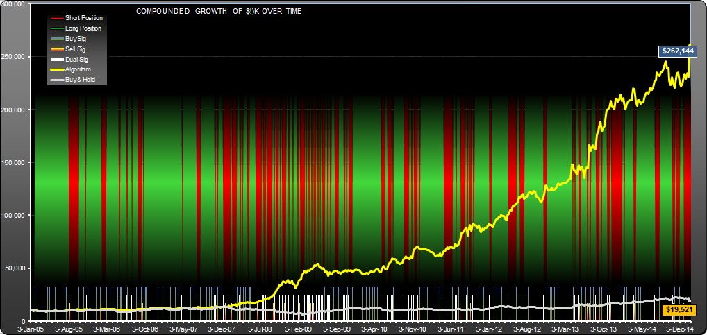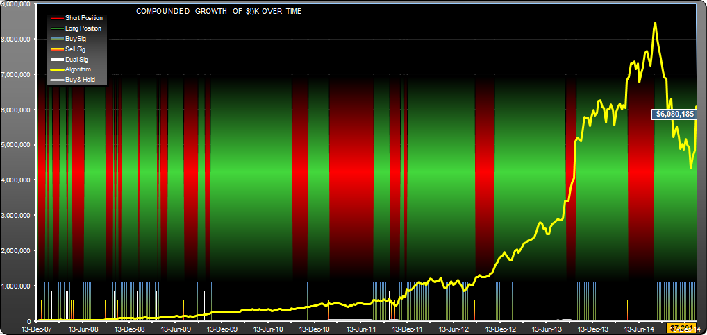
AMZN Signals (Weekly)
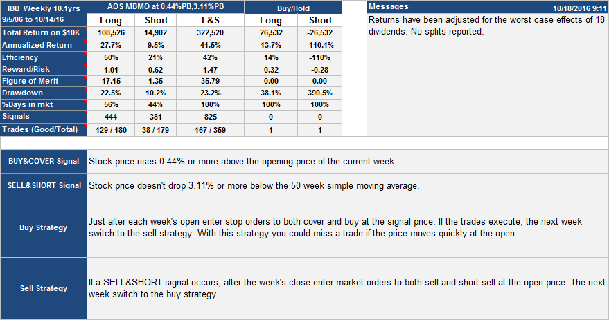
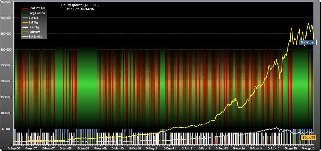
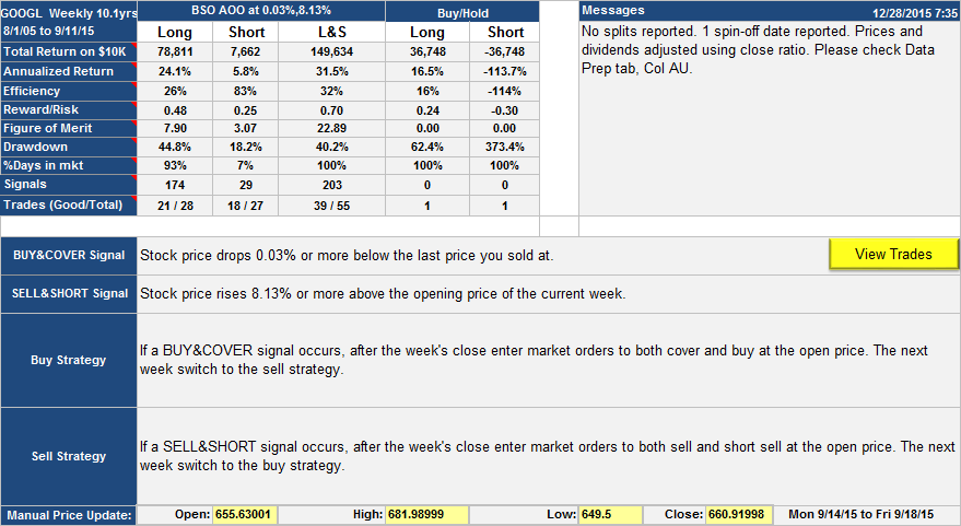
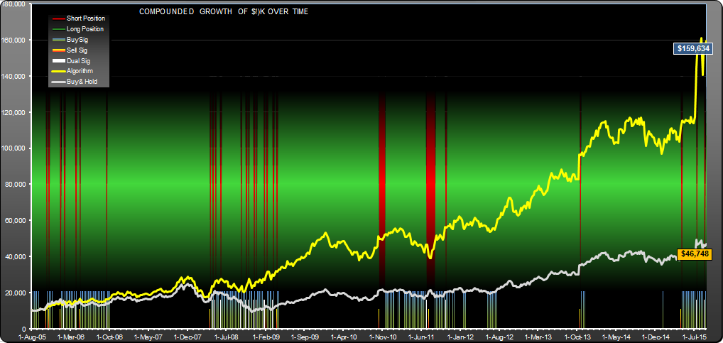
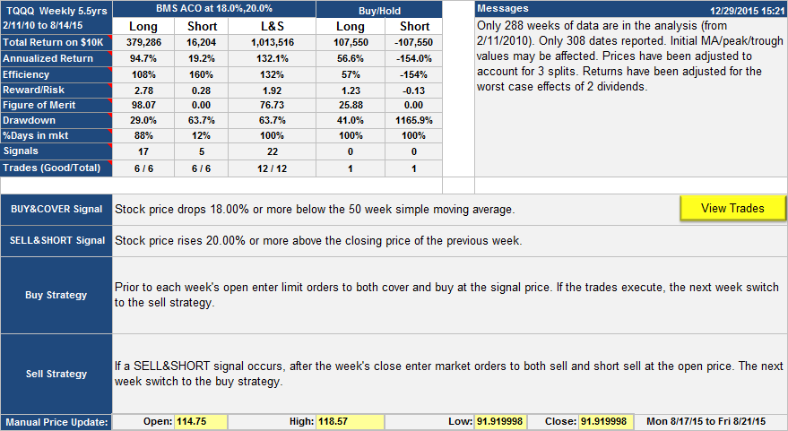
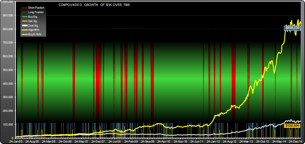
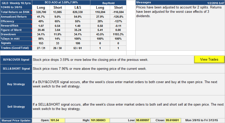
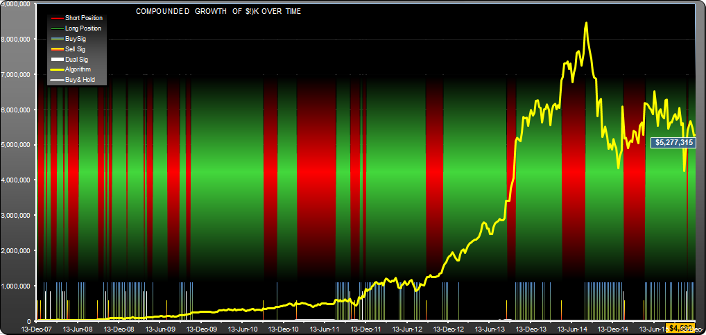
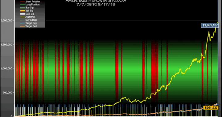
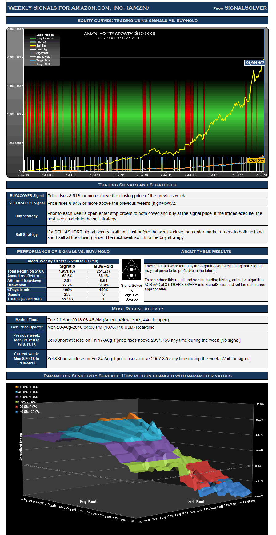
| For the 528 week (10.1 year) period from Jul 7 2008 to Aug 17 2018, these trading signals for Amazon.com, Inc. (AMZN) would have yielded $1,951,107 in profits from a $10,000 initial investment, an annualized return of 68.6%. If you had bought and held the stock for the same period the profit would have been $251,237 (an annualized return of 38.1%).
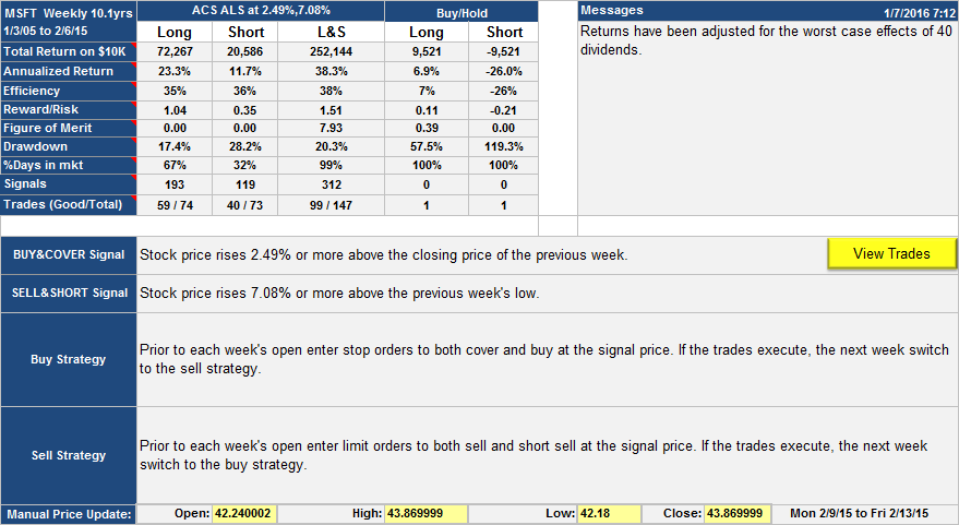
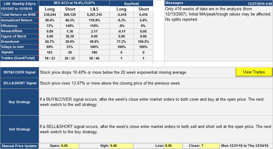
The trading style was Long & Short, meaning that you would be long or short the security at all times. For this type of strategy, not every signal is acted upon and signals are often reinforced. If you are long in the security, buy signals can be ignored, for example. Similarly if you are short you can ignore sell signals. For this particular AMZN strategy there were 198 buy signals and 55 sell signals.These led to 42 long trades of which 34 were good, and 41 short trades of which 21 were good. This is a weekly strategy, which means that weekly OHLC data is used to derive all signals and there is at most one buy and sell signal and one trade per week. Drawdown (the worst case loss for an single entry and exit into the strategy) was 29% vs. 55% for buy-hold. Using drawdown plus 5% as our risk metric, and annualized return as the reward metric, the reward/risk for the strategy was 2.01 vs. 0.64 for buy-hold, an improvement factor of around 3.2 |
, daily data")
, weekly data")
, monthly data")
, daily data")
, weekly data")
, monthly data")